Proximity & overlay analysis for upstream site selection
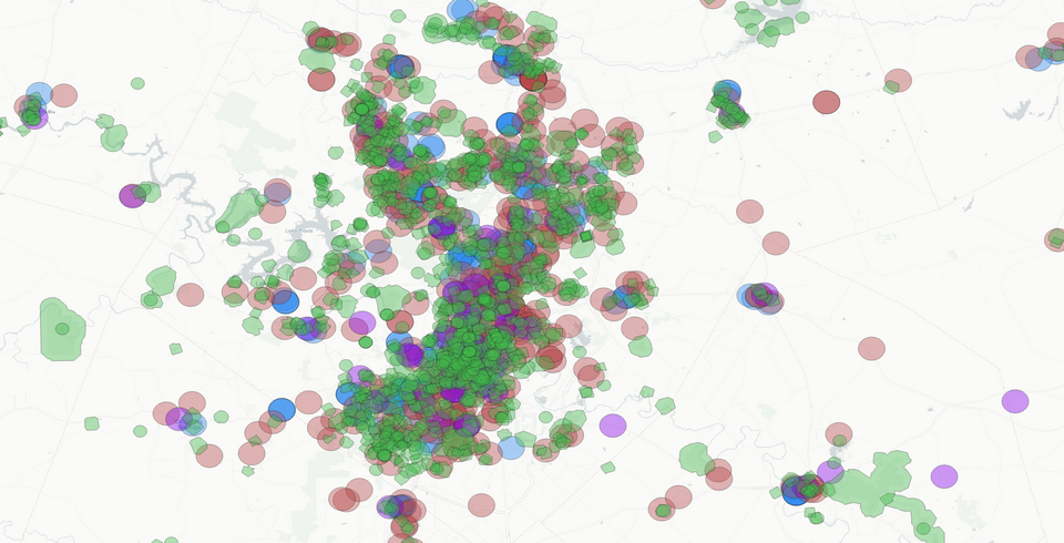
In the world of modeling, there are many ways to skin the proverbial cat. The fancier and more complex approaches get a lot of notoriety. And often for good reason.
However. There is tremendous mileage that can be gained by utilizing a handful of the simpler geoprocessing tools. And that’s what we’ll have a look at in this write-up.
We’re not splitting the atom here – just walking through some of the trusty old basics that, applied diligently, can create tremendous leverage.
We’ll walk through:
- Buffers
- Intersections
- Filtering
- Extractions
- and more
I have personally found wild value in these core spatial tools.
Let’s start by tackling a new site selection project for an undisclosed client with an aim to identify sites ripe for an undisclosed product. (Apologies for the vagueness)
Let’s start with the buy-box.
Buy-Box
Here are the broad strokes of our site requirement:
- Location: 100-mi buffer around:
- DFW
- Austin
- San Antonio
- Brownsville
- Houston
- Size: 2-5 acres
- Amenity proximity (as close as possible to):
- Grocery store
- Elementary school
- Public park
- Public library
This is our starting point – with this criteria we’ll be able to drastically reduce our prospect population from many to less (but still many).
Here's Our Approach
- Isolate our search to our given areas of interest (buffer around specified cities)
- Filter to only parcels within our acreage range
- Overlay our amenities
- Select initial proximity requirements for amenities. Create buffer zones for amenities based on the above. Evaluate results and refine as needed.
- Perform intersections between our amenity buffer zones to identify areas with a high-probability of success
- Extract parcels that fall within our intersections
- (Not shown in this write-up) filter results further and join to listing data set to categorize on-market vs. off-market parcels to generate our final prospect list
Data Sources
- AOIs: TXDoT - City Boundaries, TXDoT - Texas County Boundaries
- Land Parcels: TNRIS - Land Parcels 2023
- Schools: TEA - Schools 2022-2023
- Grocery Stores, Libraries, Parks: OSM Overpass API
Let’s get started.
First let’s spin up QGIS and get started with the Bing Virtual Earth base map. (Sourced from the Tile+ plugin for QGIS).
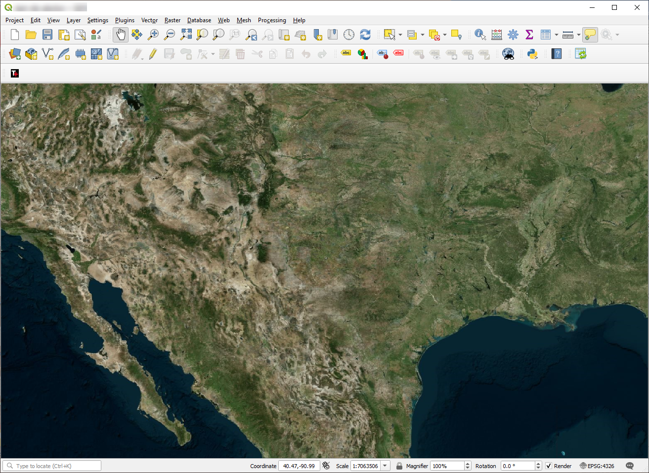
Isolate Search to Select Cities and Their Surrounding Areas
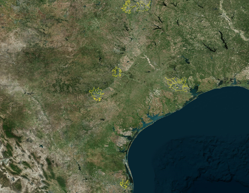
We’ll overlay our municipality boundaries and filter down to only those applicable areas.
First we'll add our TXDoT City Boundaries dataset:
Browser Pane > locate file and double-click
Then we'll filter the layer to show only
Layers Pane > Cities Layer > Filter > Filter Expression:
"CITY_NM" IN ('Austin'
, 'San Antonio'
,'Dallas'
,'Fort Worth'
,'Houston'
,'Brownsville'
)
Here are the results:
Next, let’s create our buffer zones around our cities to visualize those 100-mile buffers.
First we’ll export our cities layer to a local coordinate reference system (CRS). We’ll use EPSG: 2278 – NAD83 / Texas South Central (ftUS).
Then we’ll create our buffers.
Vector > Geoprocessing Tools > Buffer…
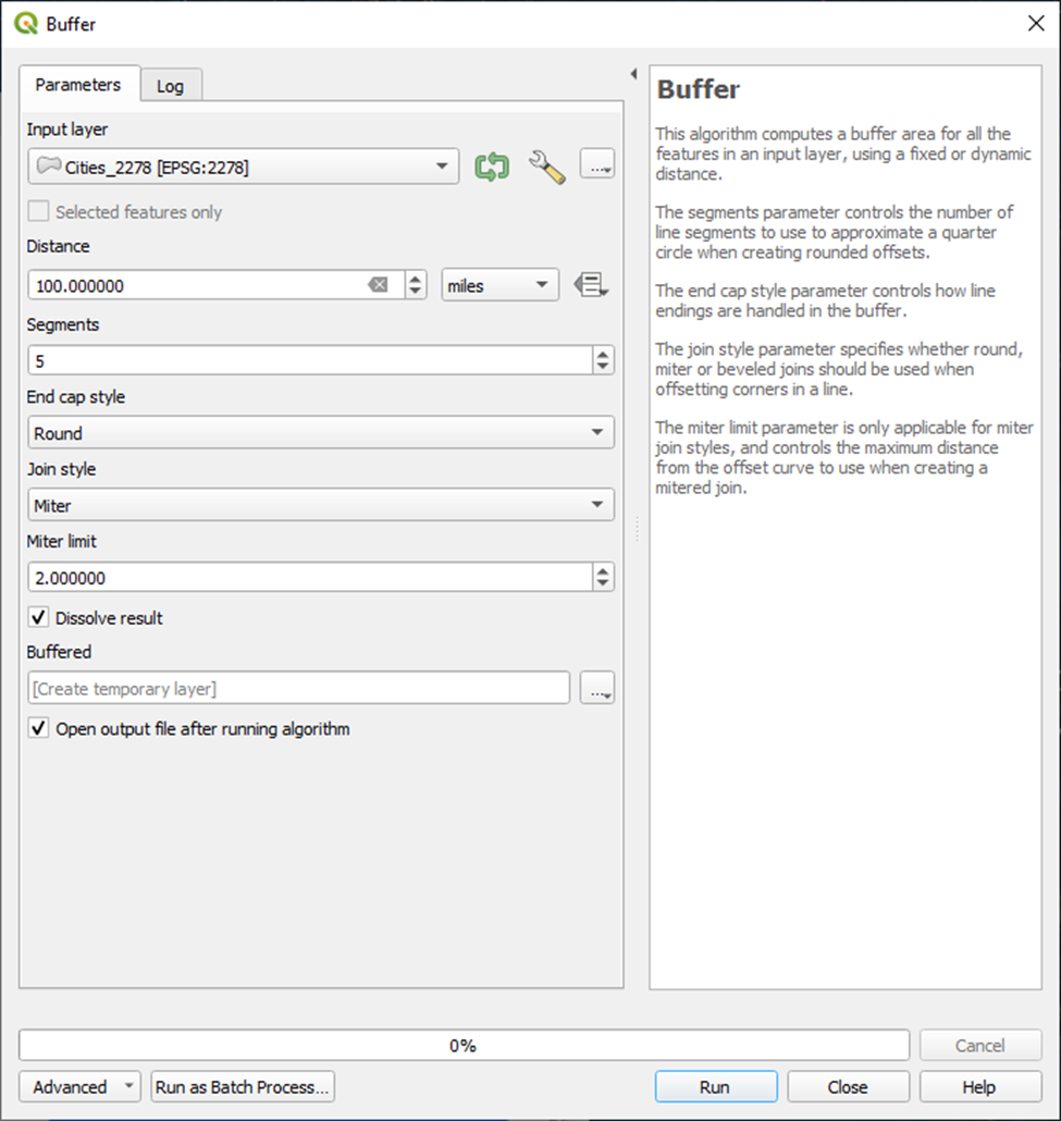
Which produces:
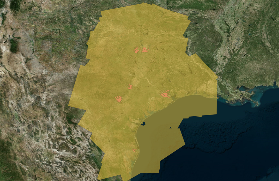
Well that’s quite a big area. Let’s create a smaller 20-mile buffer.
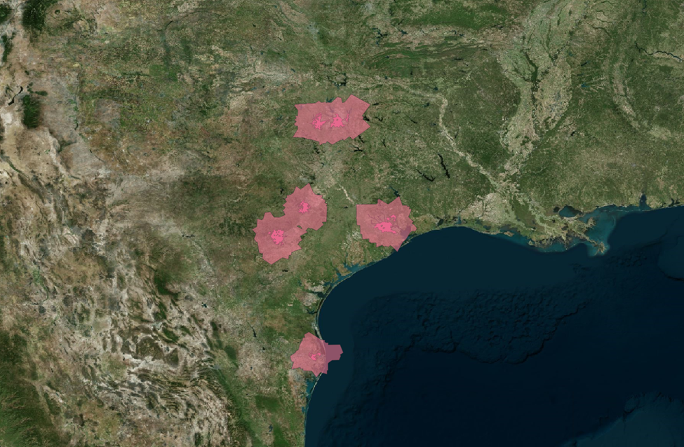
Much tighter. We’ll begin here to dial in our concept with a smaller dataset to start. We can expand out afterwards.
Alright next up, we’ll pull in our county map. We don’t have any county-specific requirements, though land parcel data is reported at a county level – so we’ll want to see which counties our buffers overlap with. This way we can pull in only the relevant land parcels.
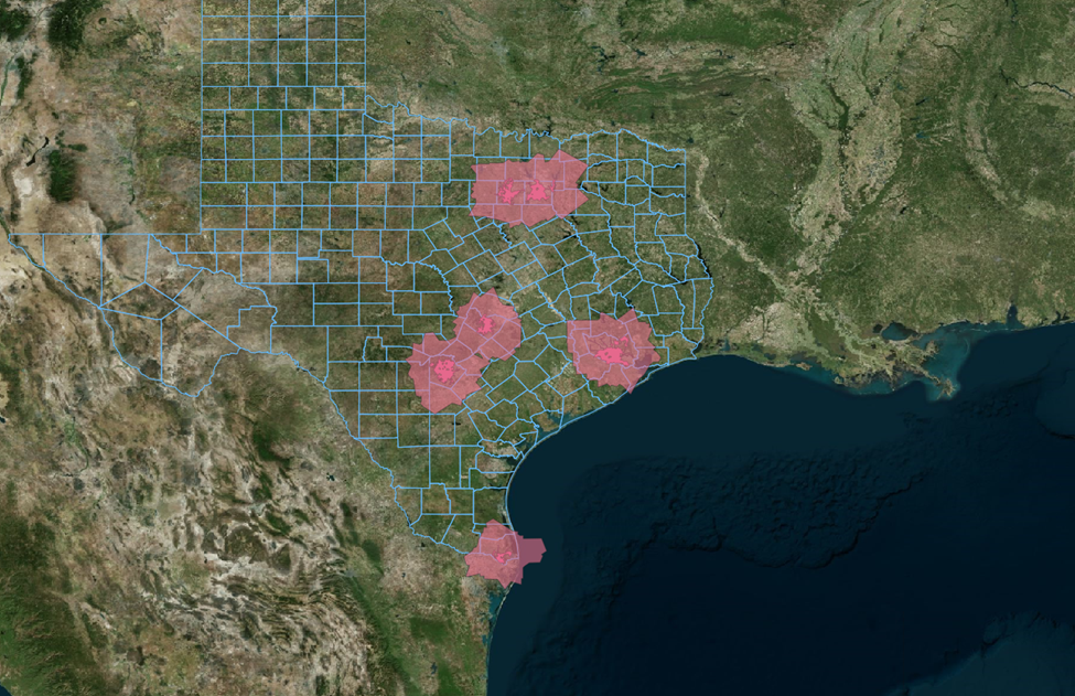
There we go. Now that’s starting to look more like Texas.
Now let’s narrow these down by extracting only the counties that intersect with our 20-mile buffer zones.
Menu Bar > Processing > Toolbox > Vector selection > Extraction by location
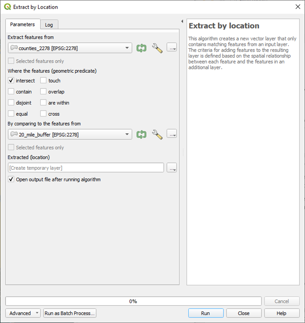
To go from this . . . to this.
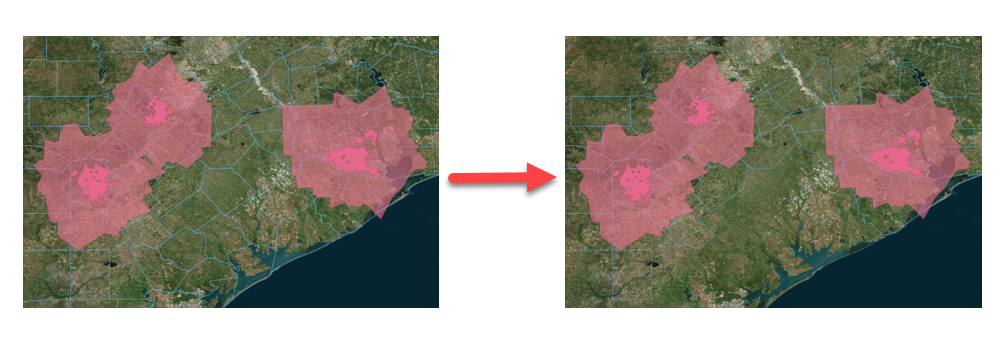
You’ll notice there are a handful of counties that intersect with our 20-mile buffer zone ever so slightly.
Our land parcel data will need to be imported individually for each county. As you can image, there are many parcels in each county – and each parcel is represented by an individual polygon.
Given that lift, I’m going to exclude the counties with little overlap.
Our aim for this first pass is to hunt for properties with a higher probability of success and we can always expand our search down the road if we have cause.
To do that we’ll:
- Turn on toggle editing: Layer > Toggle Editing
- Select Parcels to delete: Select Features by Area of Single Click > Shift + Right-Click
- Delete Selected Parcels: Delete Selected
Let’s generate our county list to pull in our parcel data.
Right-Click on your extracted Counties layer > Open Attributes Table > have a look at the CNTY_NM field.
We have 49 counties across our five different metro areas. We’ll want to tackle this in smaller pieces. Let’s focus on the counties that fall within the City of Austin buffer zone.
| FOBS_ST_CN | CNTY_NM |
|---|---|
| 48491 | Williamson |
| 48453 | Travis |
| 48287 | Lee |
| 48209 | Hays |
| 48055 | Caldwell |
| 48053 | Burnet |
| 48031 | Blanco |
| 48021 | Bastrop |
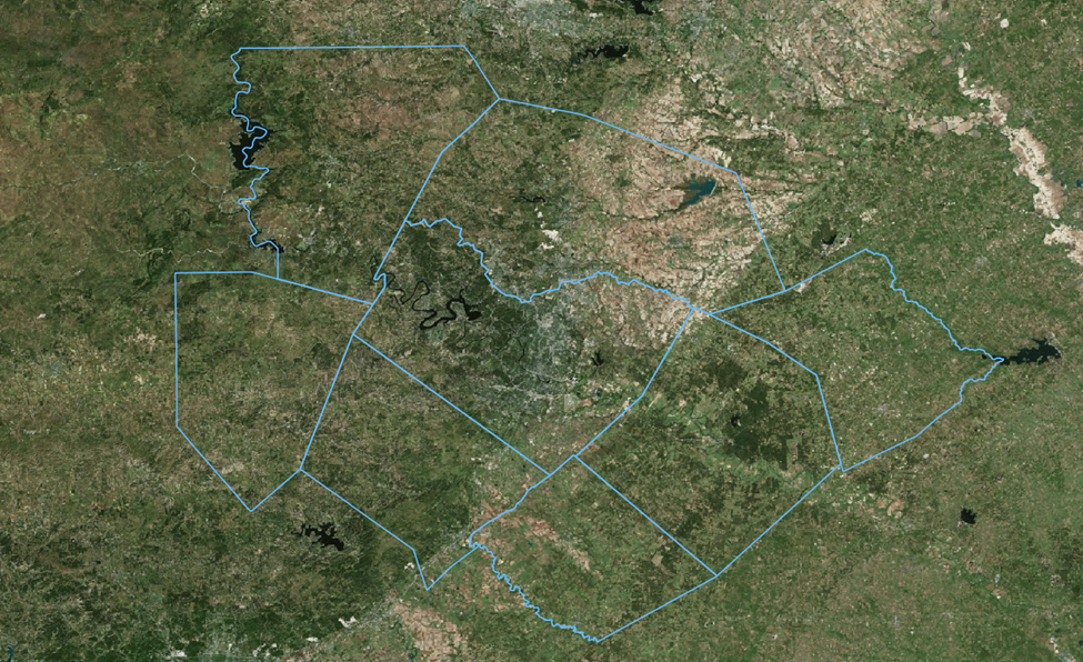
Overlay Land Parcels and Filter
Now let’s pull in our parcel data from TNRIS for these eight counties.
Travis and Caldwell counties are excluded from the TNRIS dataset so I’ll load these separately.
I have Travis County land parcels stored locally that I’ve previously sourced from the Central Appraisal District. I’m waiting on the latest authoritative version from Caldwell County. In the meantime I’ll source last years land parcel dataset from ArcOnline.
(This kind of scenario, making due with incomplete data, is not uncommon in this line of work.)
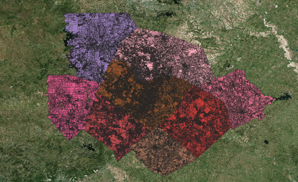
We want to make sure that each of these layers shares the same coordinate reference system and geometry type.
To do this we’ll re-project each:
• Right-click on layer > Export > Save Feature As
• Name the new vector layer
• Set the CRS (in our case EPSG: 2278)
• Set Geometry Type to Polygon
Next, we’ll narrow our land parcel selections down to only those that fall within our range of 2 – 5 acres.
We’ll start by having a look at the attribute table(s) to inspect the attributes to select our filter.
Right-Click on Layer > Open Attribute Table
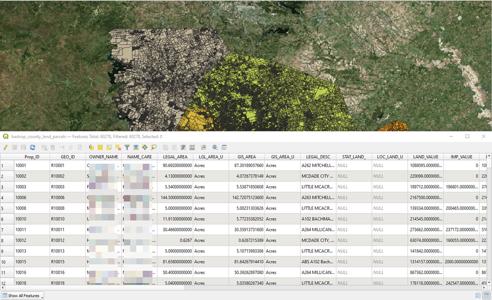
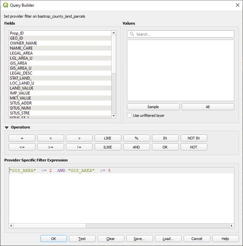
In our case we have a couple area fields to choose from: LEGAL_AREA and GIS_AREA. In my experience, it is not uncommon for Appraisal District’s reported acreage to, at times, appear a bit funny. So I am going to elect to use the GIS_AREA in this case which should be more representative of the area of the actual polygon representing the physical parcel.
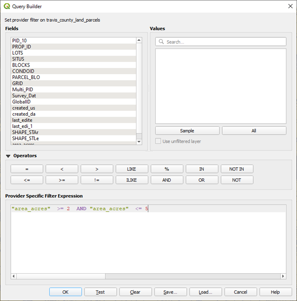
Let’s apply our filters:
Right-click on layer > Filter > Provider Specific Filter Expression
"GIS_AREA" >= 2 AND "GIS_AREA" <= 5
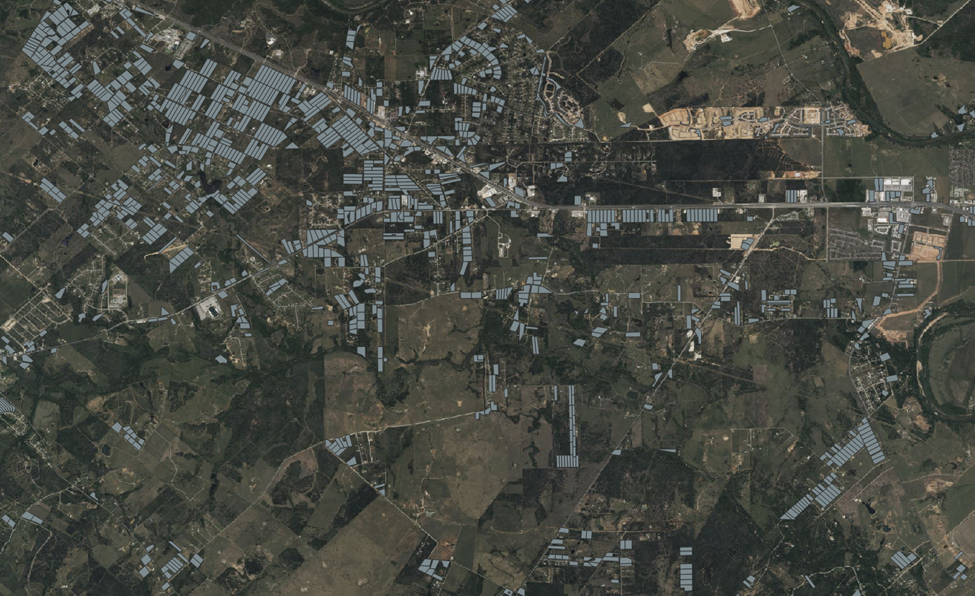
And suddenly our parcel layer is significantly more sparse:
Travis Counties dataset does not conform to the TNRIS Land Parcel Schema so we’ll need to calculate acreage ourselves.
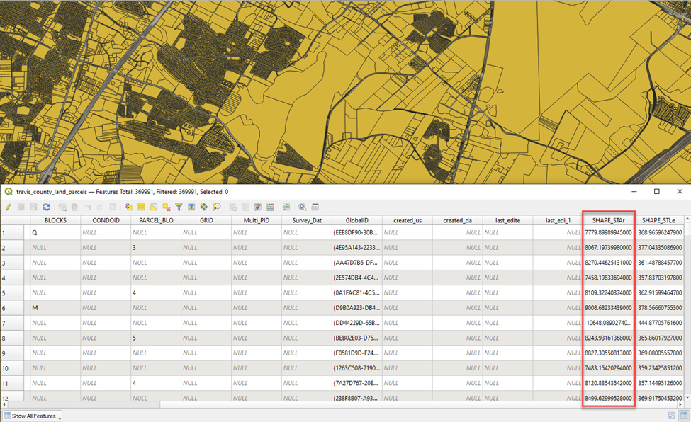
The SHAPE_STAr field in the Travis County dataset represents the area or the land parcel (reported in square feet). We’ll calculate that area in acreage my creating a new attribute field.
Right-click on layer > Open Attribute Table > Open field calculator
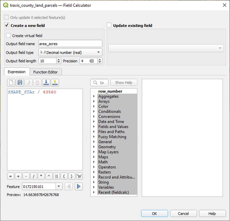
And voila.
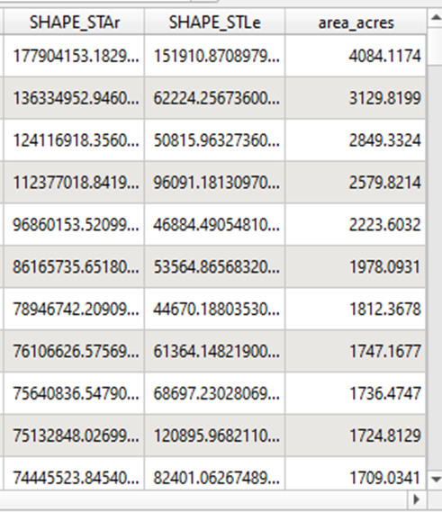
We can spot check our work by looking up a few of the Property ID’s in Travis Central Appraisal Districts Property Search portal to confirm that our acreage calculation matches theirs. Looking pretty close to me.
Now let’s add our acreage filter.
Williamson County will also require some manual calculations. Their dataset does appear to conform to the TNRIS Land Parcel schema, though the GIS_AREA field values for all records are 0 and the LEGAL_AREA column is entirely NULL.
No bueno.
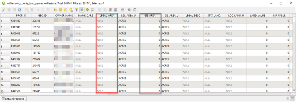
To compensate, we’ll create another field to calculate acreage manually from the polygon area. Done.
Here is the result. Not tremendously clear is it?
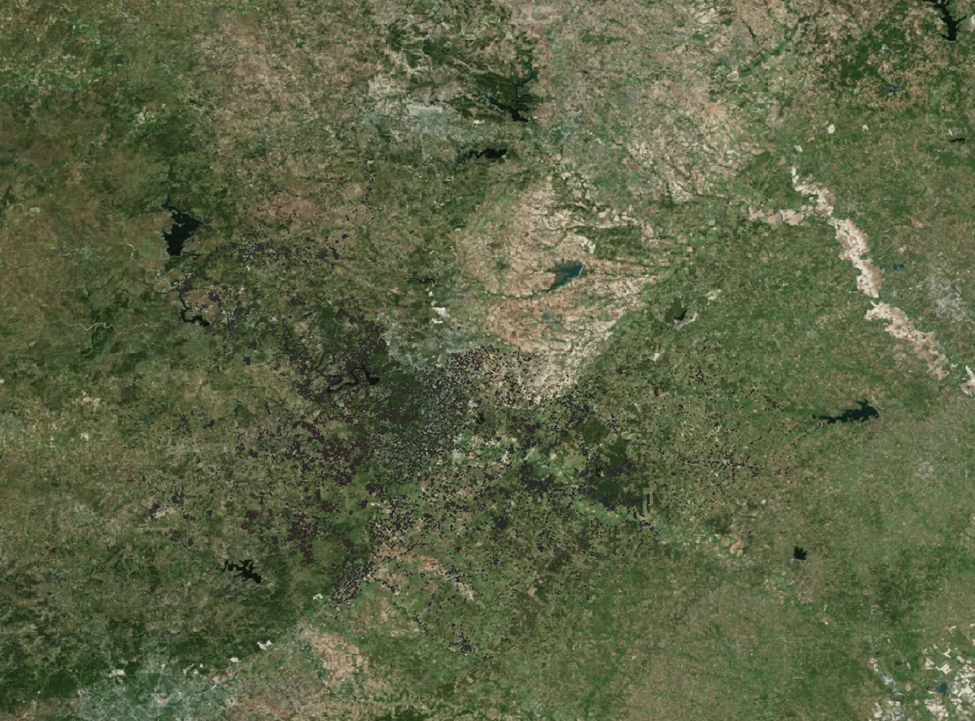
Let’s swap our base layer so we can see these somewhat more clearly.
Menu Bar > Plugins > Tile+ > Cartodb Light
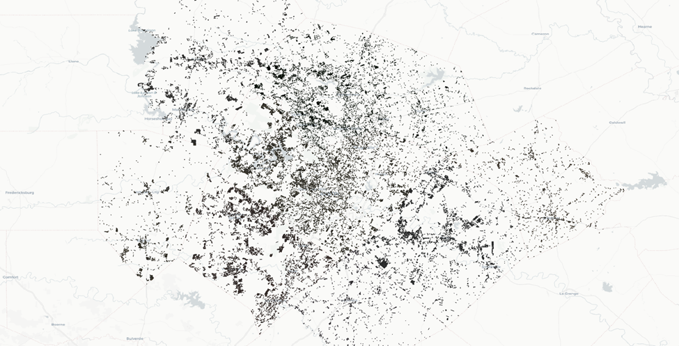
It’s not fantastic, but sufficient for the moment. We’re mapping at quite a large scale right now, but we’ll ultimately be evaluating these at a much smaller grain once we’ve whittled the dataset down.
Overlay Amenities
Amenities time. Let's start with our schools dataset.
Elementary School Layer
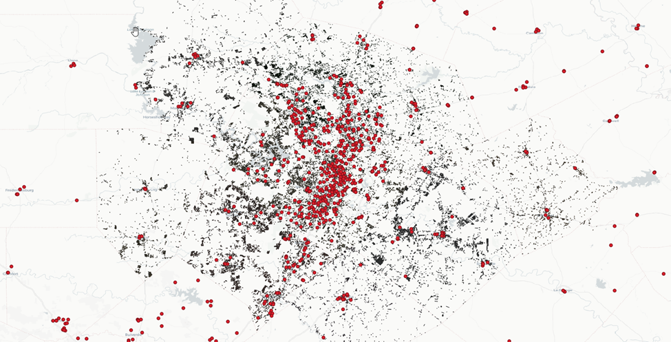
Recall that the sites we’re targeting need to have close proximity to an elementary school, specifically. Let’s filter this dataset down to visualize only elementary schools.
Filter the Schools Dataset
The TEA data set reports grade level in a text field called USER_Grade. The values for this field contain a string with the minimum grade followed by a hyphen then the maximum grade:
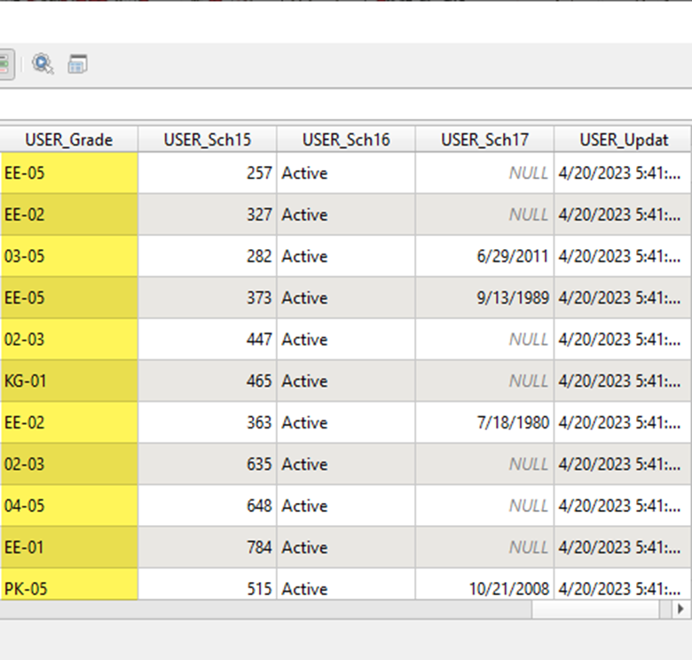
Since this field contains alphanumeric characters and hyphens we can’t do simple greater than / less than expressions like we could if minimum grade and maximum grade were reported as individual numeric columns.
Moreover, some grades aren’t numeric at all (you can see ‘EE’, ‘KG’, and ‘PK’ noted above).
Here’s our approach.
If a given range in the USER_Grade column contains at least one elementary school grade Kindergarten – 5th grade, we want to consider that a match. If it does not, we will not consider it a match.
(NOTE: I’m going to exclude schools that have a maximum grade of Kindergarten, even though it’s considered an elementary grade).
One of the easiest ways to tackle this will be to use a regular expression to find grade ranges that contain one or more of the elementary grades we’re after.
Here’s the expression that I’ve settled on:
(?<=[A-Z ]|^)(([A-Z]{2}|0[1-5]))-(0[1-9]|10|11|12|)$
Explanation:
- (?<=[A-Z ]|^): This is a positive lookbehind assertion. It checks for the presence of either an uppercase letter [A-Z], a space ' ', or the start of the string ^ immediately before the main pattern. This allows the regex to match even if there are characters or spaces before the hyphen.
- (([A-Z]{2}|0[1-5])): This is a capturing group that matches the first part of the pattern. It consists of two alternatives:
a. [A-Z]{2}: Matches any two uppercase alphabetic characters.
b. 0[1-5]: Matches the numeric values '01', '02', '03', '04', or '05'. - -(0[1-9]|10|11|12|): This part matches the second position of the pattern, following the hyphen:
a. (0[1-9]|10|11|12|): Matches numeric values from '01' to '12', inclusive. This covers valid grade values.
b. The hyphen - separates the first and second parts of the pattern.
Overall, this regular expression is designed to match grade values in a specific format (e.g., 'KG-05', 'EE-02') while ignoring any characters or spaces to the left of the hyphen. (In some cases I saw values such as ‘EE KG-05’ hence the positive lookbehind). It ensures that both the first and second parts of the grade value meet the specified criteria.
Is this solutions perfect? No. Does it get us very close? Yes.
Now let’s create a new field that uses this regex to determine if a school has elementary grades or not.
Right-click layer > Open Attributes Table > Open field calculator
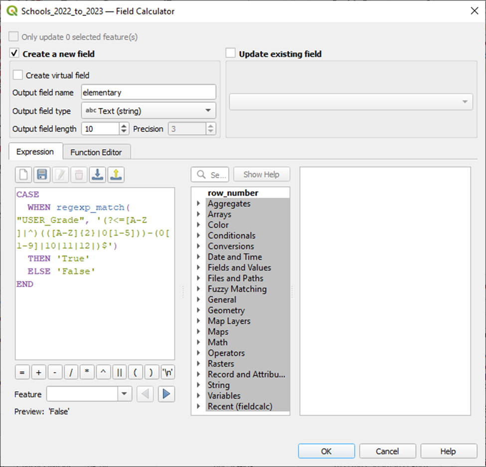
And voila.
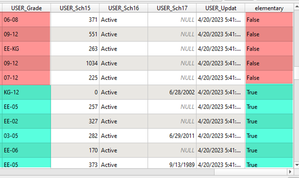
Now let’s add a layer filter based on our new elementary field.
Right-click layer > Filter
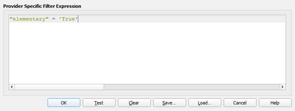
Done.
Now on to grocery stores.
Grocery Store Layer
We’ll source our grocery store dataset from Open Street Map Overpass Turbo API.
Here’s our query:
[out:json][timeout:25];
// Define Texas as a geographical area
area["name"="Texas"]->.texas;

// Gather results within the Texas area with shop=supermarket or shop=grocery
(
  node["shop"~"supermarket|grocery"](area.texas);
  way["shop"~"supermarket|grocery"](area.texas);
  relation["shop"~"supermarket|grocery"](area.texas);
);

// Print results
out body;
>;
out skel qt;
Effectively this query is pulling in all shops across Texas tagged as a supermarket or grocery. Though there’s an even easier way to do this.
You can install the QuickOSM plugin via the QGIS plugin menu to execute the above with a nice GUI.
Once QuickOSM is installed:
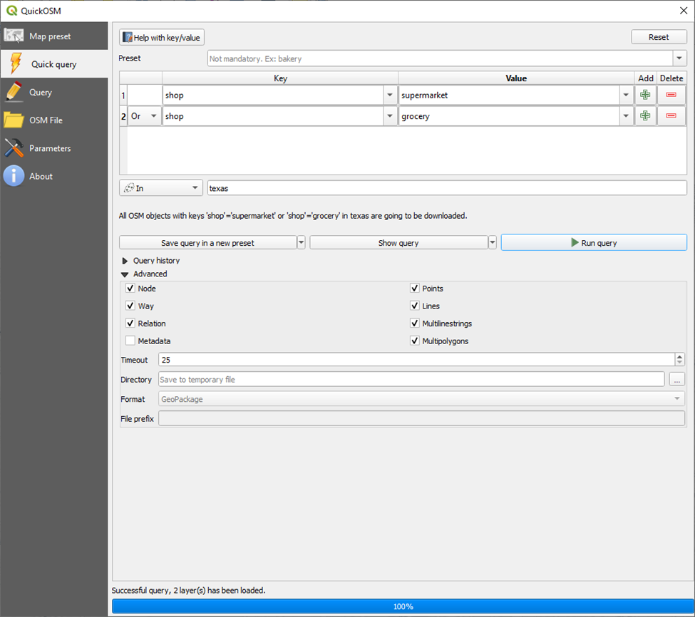
Make sure that both nodes and ways are selected to ensure the full picture. Some super markets / grocery stores are reported as nodes and others as ways, but not often both.
In QGIS the nodes will be represented as points, and the ways polygons.

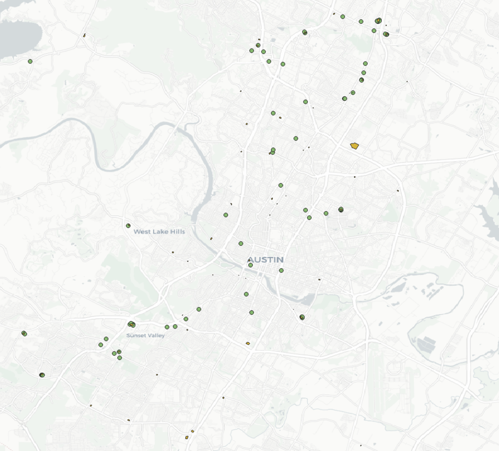
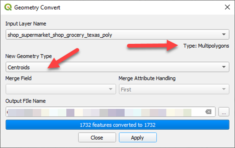
For our use case there’s no utility in polygons over points. So I’ll convert the those polygons to centroid points (representing the center points of each polygon).
We’ll use using Michael Minn’s MMQGIS plugin for this.
Convert way polygon layer to centroid points:
Menu Bar > MMQGIS > Modify > Convert Geometry Type
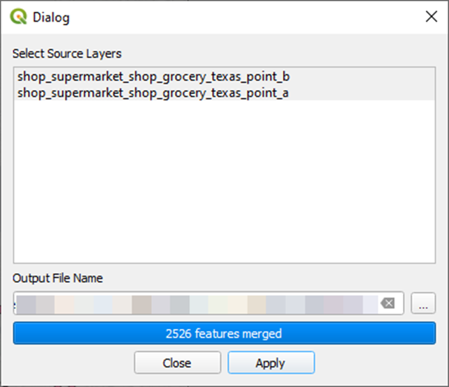
Now let’s merge our two points layers into one:
Menu Bar > MMQGIS > Combine > Merge Layers
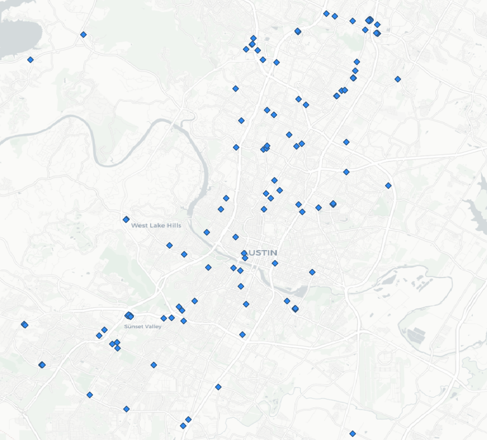
Most excellent.
We’ll repeat these steps to for libraries and parks.
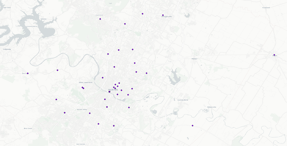
Libraries Layer
Library Quick OSM query:

Parks Layer
Park QuickOSM query:
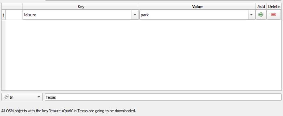
With our Parks output, however, we won’t be converting our polygon layer to centroids. The area of many parks are large enough that doing so could have a material impact on our next step – creating buffers around each of our amenities. So we’ll keep the parks point and polygon layers separate.
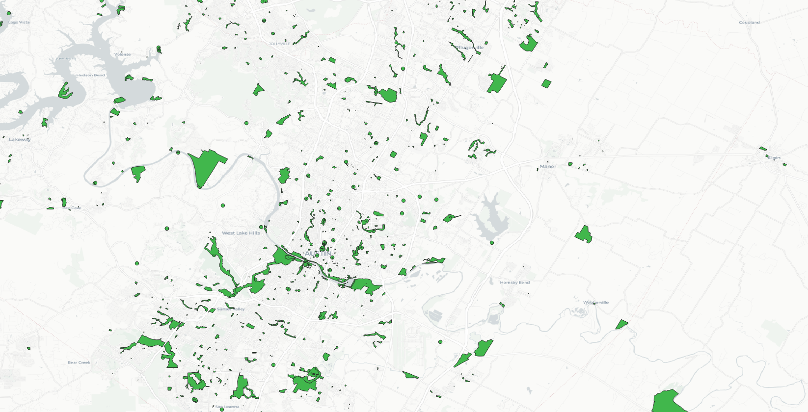
Both the parks and libraries datasets have a field that designates the type (‘public’, ‘government’, etc) – however after a quick inspection I can see that these fields are overwhelmingly NULL. Considering that and that Open Street Map is community created and not authoritative, for now we’ll skip any filtering to isolate these to ‘public’ only parks and libraries.
Now let’s have a look at all of our amenity layers together.
Combined Amenity Layers
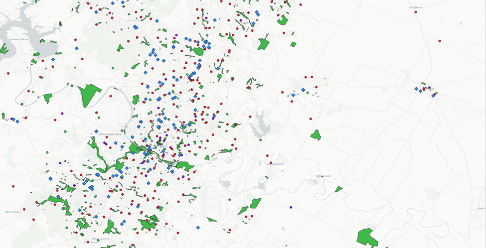
There’s a lot going on there – let’s start whittling it down to ID our most opportune areas.
Create Amenity Buffer Zones
Alright, now we have all of our layers. It’s time to start identifying which parcels fall within close proximity to our amenities.
To do this, we’ll use buffers and intersects again.
We haven’t been given a specific distance requirement for grocery, school, park, or library proximity. Rather “the closer the better”. And “if close to one of each, even better than that”
Let’s start with a half-mile for each and see where that gets us.
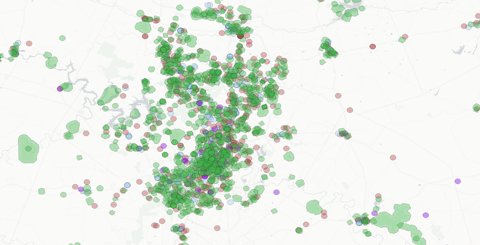
Even more going on. The park buffers seem to be plentiful (and seem to drown out the relationships between the other amenities). Let’s have a look without the parks.
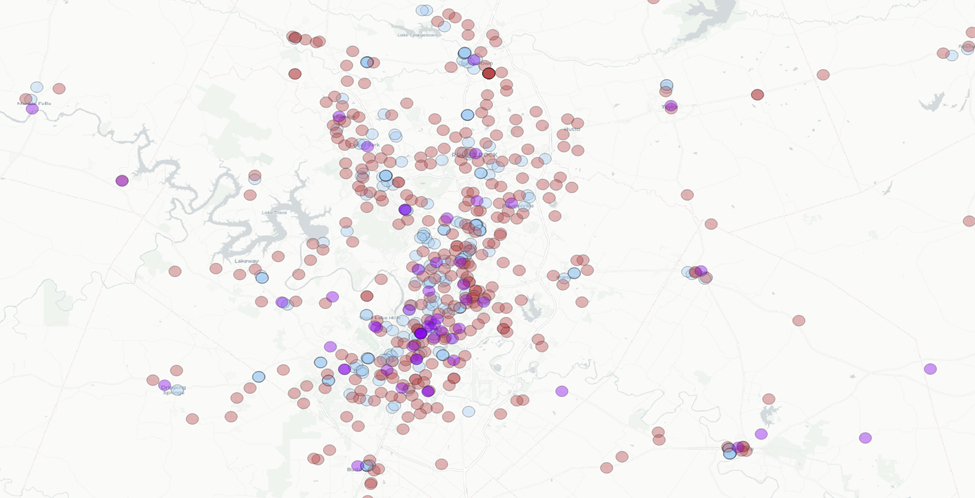
Here’s what I notice:
- There is significant coverage with the half mile park buffers
- The school and grocery half mile buffers have significant overlap in city centers. Frequently schools and grocery stores are =< 0.5 miles from one another.
- In the surrounding municipalities schools and grocery stores tend to be a bit further: not infrequently 0.5 – 1.0 miles from one another, with a handful leaning towards 1.0 mile apart or over.
- For libraries, we see a similar trend as the above two points. Though they are less frequent.
- In between municipality centers there is very little overlap.
- Schools and parks are dispersed, grocery stores and libraries tend to be anchored to city / neighborhood centers. (No big surprise there).
Let’s extend the grocery store and library buffers out to 1-mile and see what happens.
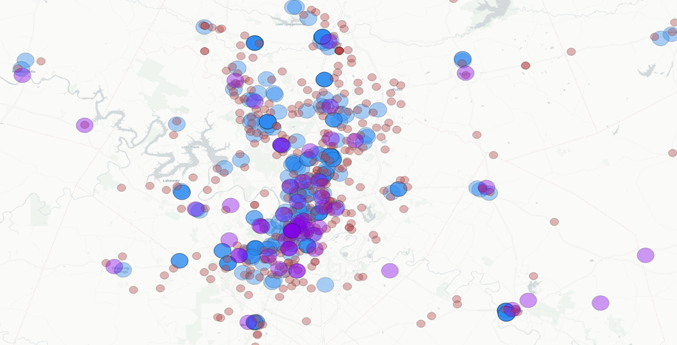
We’re now seeing lot’s of overlap of two amenities, and some strong overlap with three amenities (ignoring parks for the moment). However, if we were to delete all buffer zones except those zone with three overlaps I think we would be narrowing our search a touch too much.
I’m going to extend the schools out to a 1-mile buffer as well with the intent to get a little more area into our buffer zones with three amenity overlap.
And here we are:
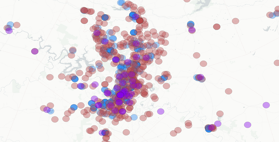
Add our half-mile park buffers back in:

Alright. I think we have something to work with here.
Create Amenity Intersections to ID Opportunity Areas
From this, I’d like to create three tiers (with increasing scores) for areas of interest:
- Overlap with school and grocery store 1-mile buffers
- Overlap with school, grocery store and library 1-mile buffers
- Overlap with school, grocery store and library 1-mile buffers AND parks 0.5-mile buffer
The theory here is that with each progression of these areas of interest (AOIs) we tighten the area but increase the probability of a near-ideal site.
Let’s start with the first – schools and grocery stores.
Menu Bar > Vector > Geoprocessing Tools > Intersection
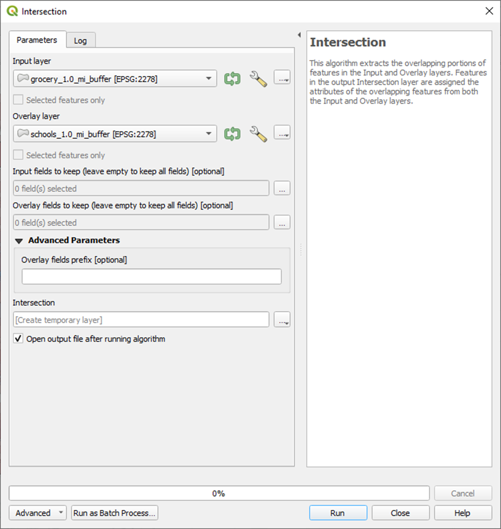
And here’s our result. These are all the areas that fall within 1 mile of an elementary school and a grocery store.
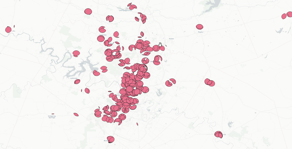
Next we’ll dissolve the results of this intersection to combine all of these separate features into one.
Menu Bar > Vector > Geoprocessing Tools > Dissolve
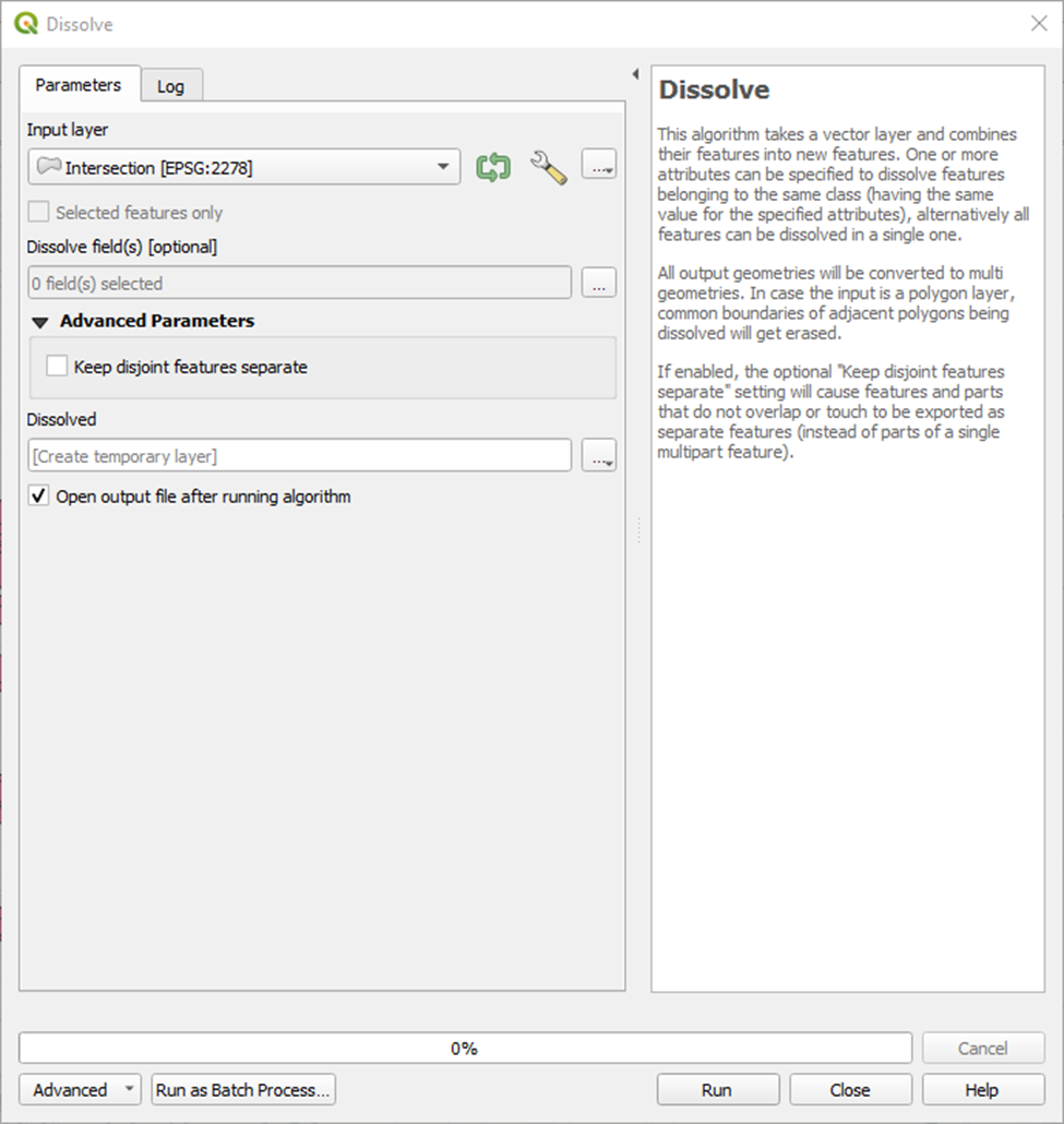
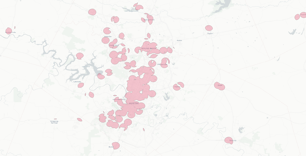
Now let’s repeat this process for AOIs two and three.
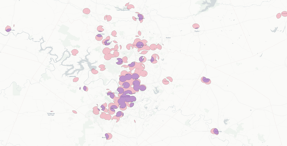
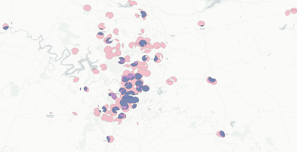
Now we have a much narrower area to work with.
Extract Parcels Within Intersections
Let’s use our narrowest AOI (with the highest probability of parcels that score well) to generate a prospect list.
Recall our parcel layers:
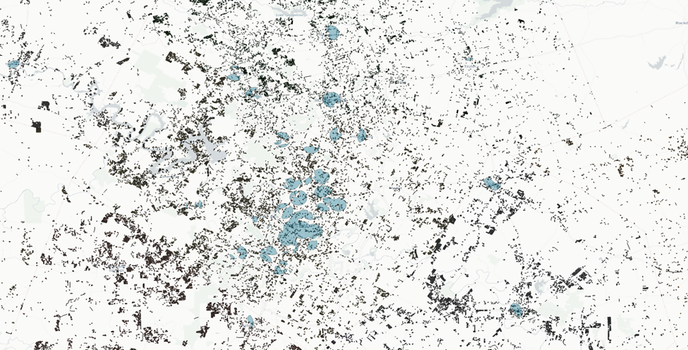
Now we’ll isolate them to only those that fall within our narrowest area of interest.
We’ll do this with an extraction by location for the respective counties.
Menu Bar > Processing > Toolbox > Vector selection > Extraction by location
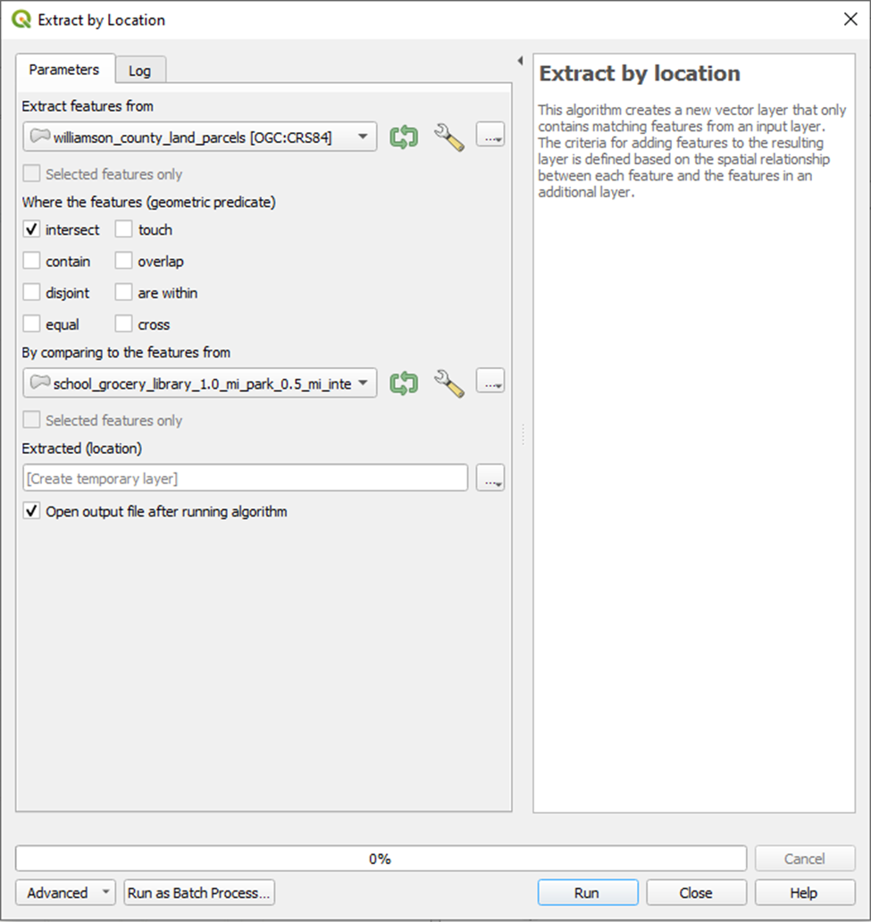
And here are our results.
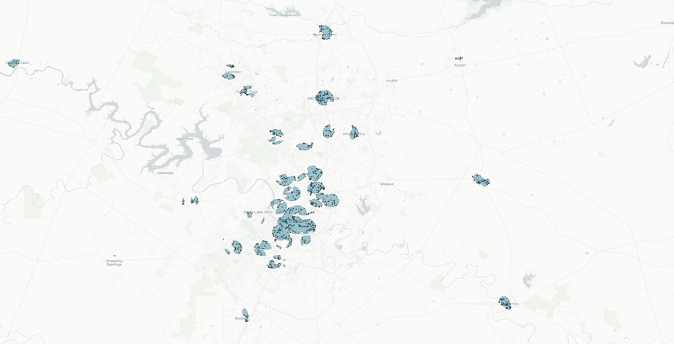
Now let’s turn on Bing Virtual Earth base map back on so we can visualize land cover and land use better.
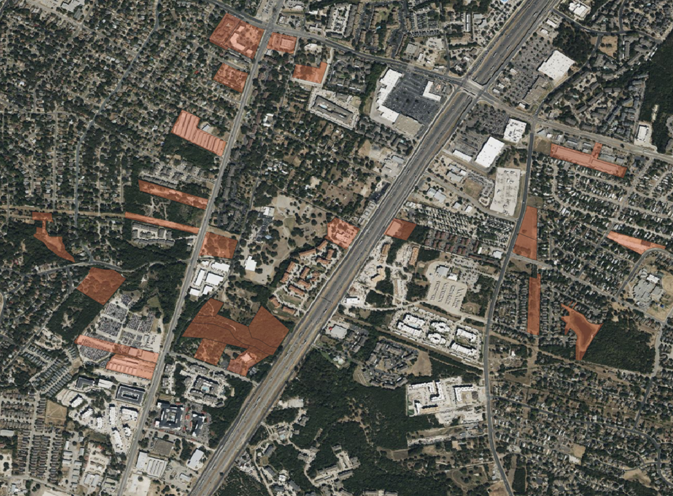
Final voila.
Wrapping Up
Here’s what we’ve generated:
- 2–5 acre parcels
- Within our Austin Metro 20-mile buffer zone
- Within 1-mile from a grocery store, elementary school and library
- Within 0.5-mile from a park
We have now taken 899,214 very low-probability parcels across the metro area and narrowed then down to 1,329 parcels with a vastly higher probability of success.
And this, I think, is a great showcase of the power of one of the most basic spatial tools – the proximity & overlay analysis.
There’s still a lot yet to do. We’ll still need to consider:
- Existing improvements
- Land use and restrictions
- Jurisdictions
- Public vs private ownership
- Utility proximity and quality
- Access
- Topography
- Flood plain
- Environmental concerns
- Areas with a particular demand for our product type
- And more
As we evaluate the results based on those factors, and rule out parcels, we may expand our area of interest incrementally to allow for more parcels that may score lower on our amenities proximity – but higher on other considerations.
Ultimately, we’ll join that final dataset to listing data to determine which of those parcels are currently (or have recently been) for sale and which aren’t. And we’ll act accordingly.
And step by step. Our haystack becomes more needles, and less hay.