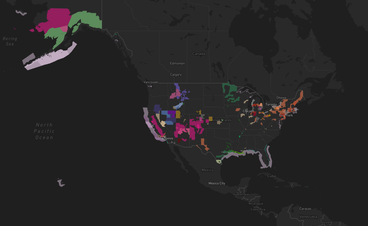
I'm not sure exactly where I first heard about Fused, but for the better part of the year it's been at the top of my LinkedIn feed.

A couple months back Isaac Brodsky and Matt Forrest walked through a few examples of how to use the tool and deliver on their tagline "Code to Map. Instantly." I've been eager check it out since, to say the least.

(Here's the LinkedIn event recording if you'd like to check it out. I'd highly recommend it).

In my case the timing of all this was pretty serendipitous. I've been wrestling with soul-sucking infrastructure decision overload. To-date pretty much any analysis, map, or data app that I've built has been done locally. That's where it starts and that's where it ends. This has made sharing my work with anyone quite difficult (including myself if I'm away from my desktop).

I've recognized that cloud deployment is something I need in my life.

But I want to do it efficiently, with minimal storage and compute expense, I don't want to be backed into a vendors corner, and frankly I don't want to spend much time learning about deploying and optimizing infrastructure. (I'd rather be mapping stuff).

Turns out this is exactly what Fused offers. Lucky me 😁

Fused in a nutshell

I'm going to plagiarize a bit here copy and paste the highlights that got me intrigued:

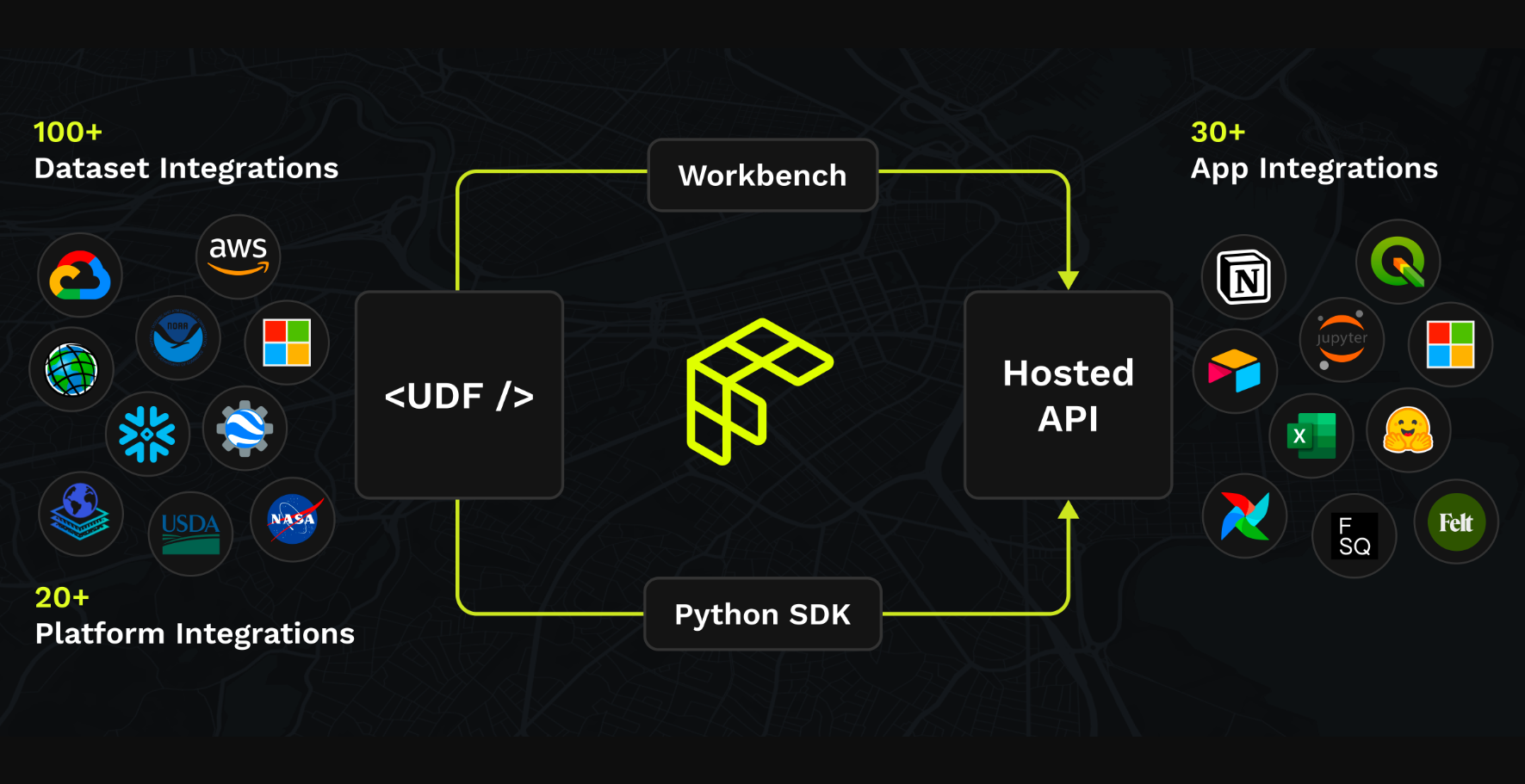
Fused is the glue layer to run workflows to load data across your most important tools.

Run real-time serverless operations at any scale and build responsive maps, dashboards, and reports.

Develop in production. Run on any scale data without infra friction.

Avoid vendor lock-in. Bring interoperable workflows, apps, and maps to your preferred stack.

At the core of Fused, is the User Defined Function (aka UDF). It's the Pythonic wrapper where you define the logic to:

1. Ingest things
2. Process things
3. Then return the results of things

It's a Python function.

The super cool thing about the Fused UDF is you define it once and the result is a hosted API endpoint that executes on a serverless machine when you call it, returning the output you defined.

You can feed endless data & parameters into it (within the bounds of your defined logic) for processing and your downstream apps, maps, models, pipelines and IDEs can fetch the results.

Pretty cool huh?

National Weather Service hazards

I wanted to select a simple use-case to start getting familiar with the Fused Python-SDK and Workbench.

The National Weather Services (NWS), which rolls up to the National Oceanic and Atmospheric Administration (NOAA), provides some very useful datasets that are pertinent to just about all of us (in the U.S. and it's territories).

When you get those "Emergency Alert. Flash Flood Warning." notifications on your phone - that's these guys.

Their Watch, Warning, and Advisories (WWA) aka Hazards MapServer reports on those hazards that drive the alerts that drive those notifications.

Those hazards come in 3 broad flavors:

And 124 specific Hazard Types:

As you can imagine - there are quite a few different use cases where mapping these would be useful. For example, assessing proximity and potential hazard to:

• Critical infrastructure
• Hospitals
• Emergency services
• A real estate portfolio

Getting familiar with the FeatureServer

The ArcGIS REST service offers a WWA FeatureServer endpoint. We'll select this path to fetch our data.

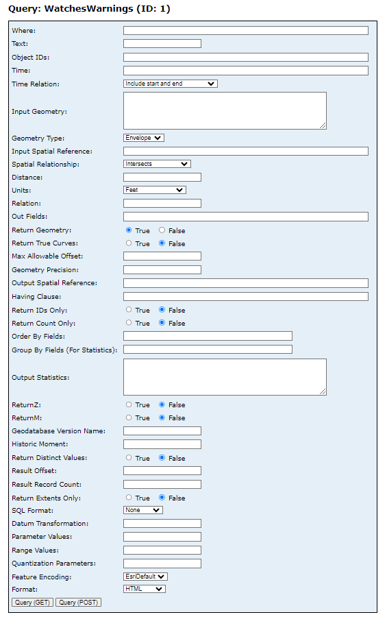
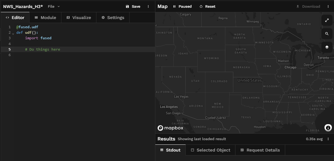
Now let's construct our call. We'll start with the Fused flavored skeleton of a UDF in Workbench.

Next we'll import the requests library, construct our arguments, make our GET request and fetch our data and cache the results with the nifty @fused.cache decorator to persist the results across runs.

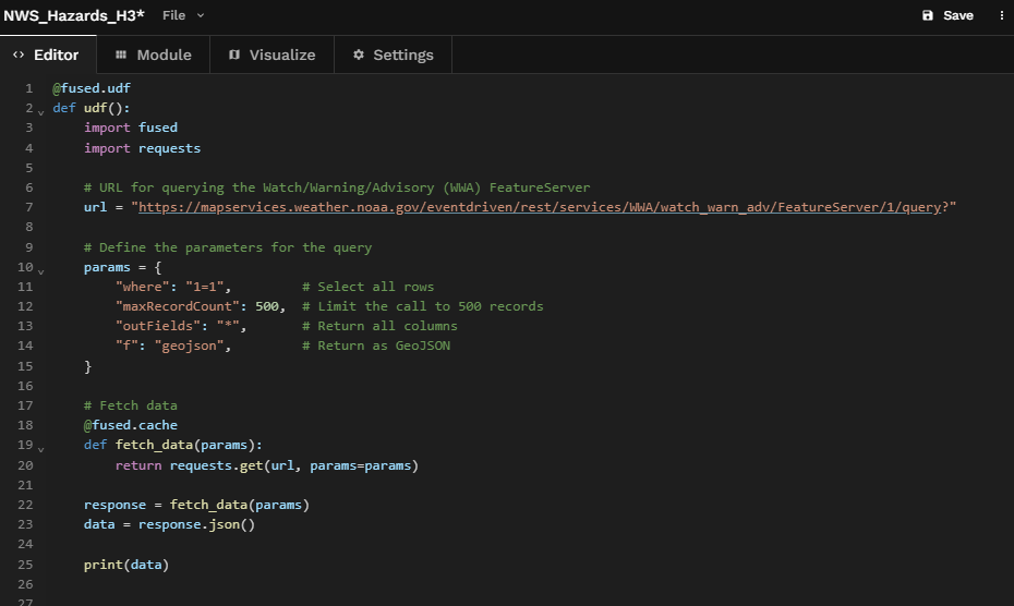
And we'll print our data just to make sure we got something.

Got something 👌.

Mapping hazards with GeoPandas

Now let's map the data we've fetched.

We'll import geopandas, convert our GeoJSON data to a GeoDataFrame with our CRS set to "EPSG:4326", and then we'll return the gdf.

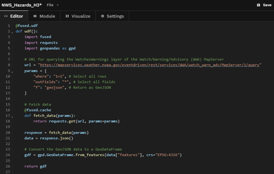
And just like that our hazards come to life.

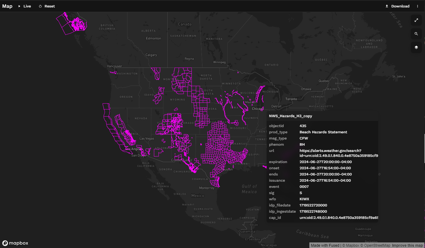
We could stop right here

In 26 lines of code and less than 5 minutes we've now built a full-blown (albeit very simple and unenriched) UDF.

If we were satisfied with this and wanted to pull it into another app or map we'd click Save, hop over to the Settings tab, and generate a signed URL and now we have our very own hosted API endpoint.

But let's make it a little better.

Project polygons to H3 cells

Now it's very unlikely that you would do any of this work to just view NWS Hazards. If that's all you wanted to do, you'd just visit their web map.

It's more likely that, like me, you'd like to relate this Hazard data to some other data. Likely in the form of point lookups, spatial joins, distance calculations, etc.

To that end - we can optimize the data product we're producing by converting our gdf geometries to H3 cells. Now we probably won't see incredible performance gain with a dataset of this size (quite small). But large datasets could benefit tremendously from it when it comes to performing subsequent (now less expensive) operations on that data.

Frankly, I just wanted an excuse to play with H3 cells in this direction (filling polygons with cells vs aggregating points to cells).

Let's take a quick commercial break to hear from our (not a sponsor) H3

I imagine most folks that are reading this and have made it this far down are already familiar with H3. But in case you're not, here's a few highlights (scraped from their site) for why it's something worth looking into.

H3 is a hierarchical geospatial index.

H3 was developed to address the challenges of Uber's data science needs.

H3 can be used to join disparate data sets.

In addition to the benefits of the hexagonal grid shape, H3 includes features for modeling flow.

H3 is well suited to apply ML to geospatial data.

They've partitioned Earth into hexagons at 16 different resolutions. Each hexagon has exactly 6 neighboring cells and the distance from the center of each cell to it's neighbor is identical. From what I understand, this creates significantly more uniformity and is much less prone to distortion and edge effect bias seen in other grid systems.

My takeaway is it's powerful and something to become familiar with 🙂.

Back to filling our polygons with hexagons

The latest (v4.0.0 beta) release oh h3-py offers some improved methods for performing our polygon fills. You can install it with pip install h3 --pre or with pip install 'h3==4.0.0b3'. Let's add it to our UDF.

We'll use:

• geo_to_cells() to translate our gdf Shapely geometries to H3 cells
• cells_to_h3shape() to translate our cells to H3Shape (valid geometry objects in the eye of GeoPandas)
• And we'll replace our gdf Shapely geometry values with our new H3Shape geometry objects

The documentation on all that can be found here.

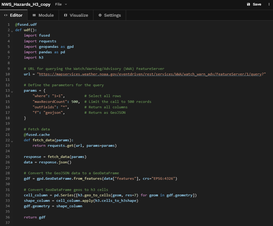
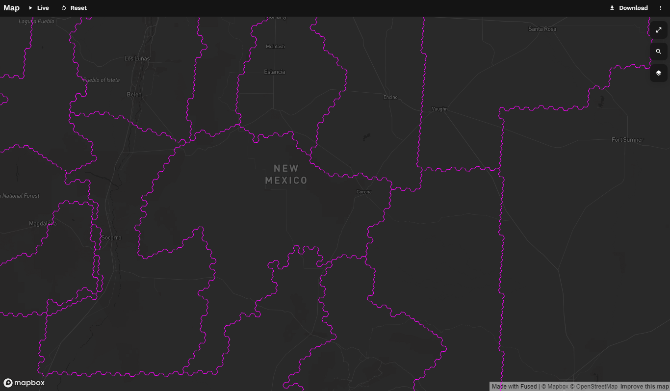
And the result is a bunch of hexagons.

Picking an H3 resolution

Now, I picked Res 7 here (res=7 line 28). This resolution has an approximate area of 5.2 km² (cell resolution table here). Why did I select this resolution?

It felt like a good guess.

I've read that Uber most often used Res 9 (0.1 km²) which is roundabout an average city block. Makes sense for their use case. For mine here, we're dealing with much bigger area.

Here's roughly the same bounding box at Res 4:

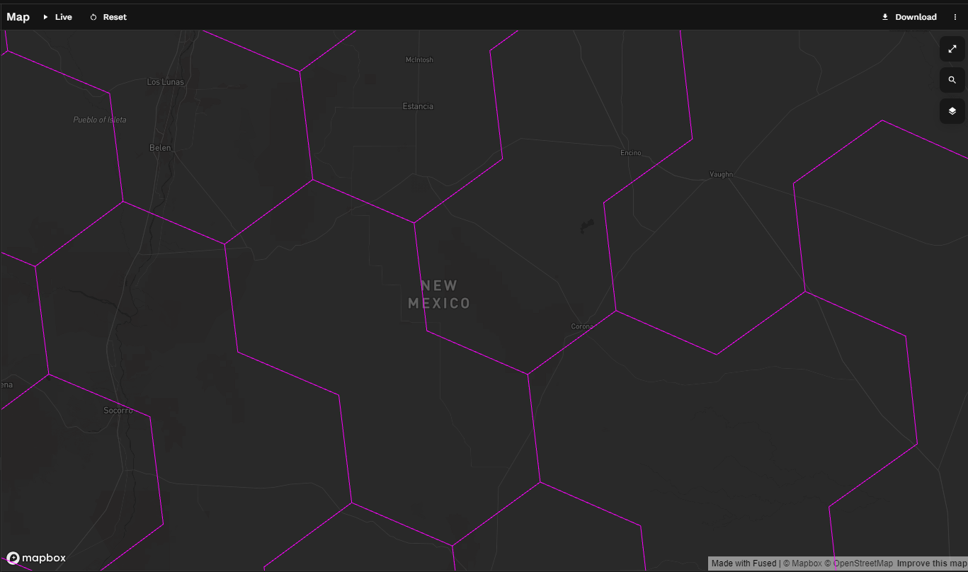
Selecting a resolution is a tradeoff. At a higher resolution your edges more accurate represent the lines of the polygon you're trying to fill, but the processing is more expensive.

Here's a fun Observable notebook by Nick Rabinowitz that illustrates that tradeoff.

My first takeaway on this topic is that resolution should be selected within the context of your use case.

(and in this example we haven't arrived at that use case yet)

My second takeaway (thanks to my new internet friend David Ellis) is that you can and should evaluate fallout at different resolutions in the context of a particular use case. From David when I asked "how do I pick the right H3 resolution?":

A rule of thumb from my (brief) EE days is if the impact on the signal is less than three orders of magnitude (less than 0.1%) then you can basically ignore it for practical purposes. So if you do the analysis for a single one of these geofences the classic way and compare against your H3 version at res 7 and the difference is below 0.1% you should be fine.

So Res 7 results in a 2.4% loss but Res 8 results in a 0.087% loss, then Res 8 is probably the winner.

Which brings me to the next point.

Add user-defined variables

The correct resolution will vary based on use case, so let's let the user pass whatever resolution they like into the UDF. And while we're at it, let's add a coupe more arguments.

We'll add the following arguments to our UDF:

• A bounding box to make the UDF capable of tiling: bbox: fused.types.TileGDF = None
• CRS (or coordinate reference system): crs="EPSG:4326"
• And our H3 Res:res=7

Tiling

We'll also add some additional params to pass our bbox to the FeatureServer so we can tile our map.

By doing this, we're dynamically fetching only the subset of the data we care about (we're not loading features from Alaska if we're only viewing Texas).

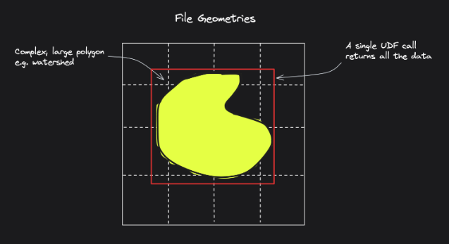
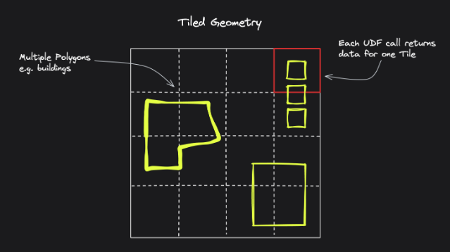
By default, 1 tile = 1 API call. And we can make those single tile calls in parallel.

Here's Fused's illustration of Files vs Tiles:

To pass the bounding box to ArcGIS FeatureServers we'll need to do a little manipulation. Here's what my selected fused.types.TileGDF bbox yeilds:

To easily translate this to one of the acceptable ESRI bbox geometry formats envelope we'll use the below to convert it to the desired structure.

Which, for our New Mexico area above, yields an envelope like:

Now here's all those updates strung together (shifting to code blocks now - too many lines for images):

@fused.udf
def udf(bbox: fused.types.TileGDF = None, crs="EPSG:4326", res=7):
    import fused
    import requests
    import geopandas as gpd
    import pandas as pd
    import h3

    # Generate ESRI-friendly envelope bbox
    total_bounds = bbox.geometry.total_bounds
    envelope = f'{total_bounds[0]},{total_bounds[1]},{total_bounds[2]},{total_bounds[3]}'

    
    # URL for querying the Watch/Warning/Advisory (WWA) FeatureServer
    url = "https://mapservices.weather.noaa.gov/eventdriven/rest/services/WWA/watch_warn_adv/FeatureServer/1/query?"

    # Define the parameters for the query
    params = {
        "geometryType": "esriGeometryEnvelope",  # Type of geometry to use in the spatial query (for bbox)
        "geometry": envelope,                    # The bounding box geometry for the query
        "inSR": "4326",                          # The spatial reference of the input geometry
        "spatialRel": "esriSpatialRelIntersects",# Spatial relationship rule for the query
        "returnGeometry": "true",                # Whether to return geometry of features
        "where": "1=1",                          # SQL where clause to filter features (no filter here)
        "maxRecordCount": 500,                   # Maximum number of records to return per request
        "outFields": "*",                        # Fields to return in the response (all fields)
        "outSR": "4326",                         # The spatial reference of the output geometry
        "f": "geojson",                          # Format of the response (GeoJSON)
    }

    # Fetch data
    @fused.cache
    def fetch_data(params):
        return requests.get(url, params=params)

    response = fetch_data(params)
    data = response.json()

    # Convert the GeoJSON data to a GeoDataFrame
    gdf = gpd.GeoDataFrame.from_features(data["features"], crs=crs)
    
    # Convert GeoDataFrame geos to h3 cells
    cell_column = pd.Series([h3.geo_to_cells(geom, res=res) for geom in gdf.geometry])
    shape_column = cell_column.apply(h3.cells_to_h3shape)
    gdf.geometry = shape_column

    return gdf

Addressing tiling and record count concerns

There are a couple scenarios, likely to occur, that our current implementation does not account for:

1. Situations where there are "too many" features for a given tile
2. Situations where there are no features for a given tile

Let's account for both.

To keep the main body of our UDF clean and focused on the business logic, we'll put this more utilitarian helper logic in the Module tab in workbench which will ultimately produce a utils.py file that we'll import into our primary UDF.

Now, considering our first concern listed above we need to be aware of a couple things:

• Advertised limits on the number of records we can fetch from an API (in the case of this FeatureServer the advertised limit was maxRecordCount = 2000)
• ... and effective limits. I noticed that calls to this server started sporadically failing around ~700 records (hence our param of "maxRecordCount": 500)

Now by tiling this UDF we dramatically reduce the frequency of running into this issue since each tile represent a single call. It is far less likely that we'll exceed our max record count for a single tile vs attempting to fetch all hazards by implementing the UDF as a single file call.

Nonetheless, we want to be able to handle those situations when they arise. To do that, we'll implement pagination.

What that means is if the number or available features exceeds our maxRecordCount we'll simply make multiple calls and keep track of where we left off in between. In our example, if there are 1,322 features available for a tile we'd make 3 calls for it:

• Call #1: 500 records
• Call #2: 500 records
• Call #3: 322 records

We'll combine these and return them.

To handle the second scenario (where there are no features for a given tile) we simply return None or alternatively and empty geodataframe.

Here's how we implement all that (in our utils.py file):

import fused
import pandas as pd
import geopandas as gpd
import requests

@fused.cache
def fetch_all_features(url, params):
    """
    Fetch all features from a paginated API. Makes multiple requests if the number of features exceeds maxRecordCount of a single call.

    Args:
    url (str): The API endpoint URL.
    params (dict): The query parameters for the API call, including 'maxRecordCount'.

    Returns:
    list: A list of all features retrieved from the API.
    """
    
    all_features = []
    max_record_count = params["maxRecordCount"]
    
    while True:
        response = requests.get(url, params=params)
        if response.status_code == 200:
            data = response.json()
            if "features" in data and data["features"]:
                all_features.extend(data["features"])
                if len(data["features"]) < max_record_count:
                    break
                # Update params for the next page
                params['resultOffset'] = params.get('resultOffset', 0) + max_record_count
            else:
                break
        else:
            print(f"Error {response.status_code}: {response.text}")
            return None
    return all_features

Add a colormap for better eyeballing

Almost done.

One clear improvement is we can map specific colors for each of our hazard types so we can quickly spot what kind of hazards are occurring where. The NWS Weather & Hazards Data Viewer uses a particular colorway for their Hazards data.

We'll produce a dictionary CMAP that maps each Hazard Type key to it's respective RGB color values.

We'll then create a helper function to add these r,g,b values to our gdf.

We'll handle this in the Module tab as well.

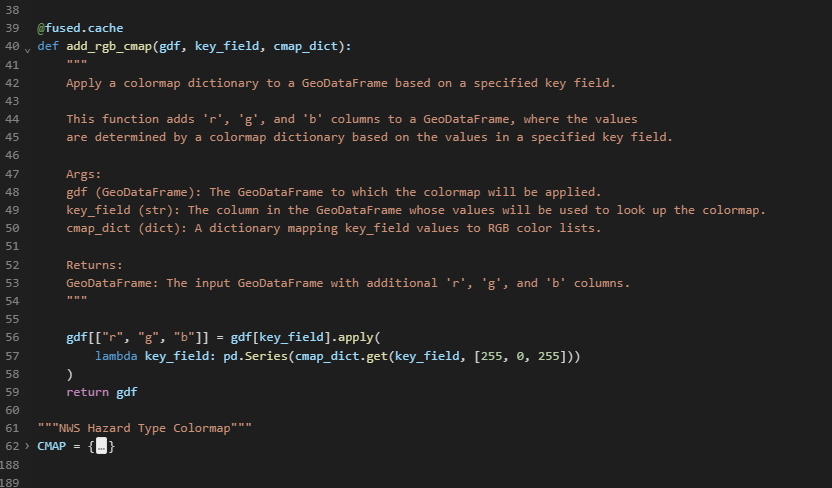
We'll import our utilities (fetch_all_features, add_rgb_cmap , and ourCMAP) to our NWS_Hazard_H3.py editor and update our code slightly to call them.

Here it is.

@fused.udf
def udf(bbox: fused.types.TileGDF = None, crs="EPSG:4326", res=7):
    import fused
    import pandas as pd
    import geopandas as gpd
    import h3
    import requests
    from utils import fetch_all_features, add_rgb_cmap, CMAP


    # Generate ESRI-friendly envelope bbox
    total_bounds = bbox.geometry.total_bounds
    envelope = f'{total_bounds[0]},{total_bounds[1]},{total_bounds[2]},{total_bounds[3]}'
    
    # URL for querying the Watch/Warning/Advisory (WWA) FeatureServer
    url = "https://mapservices.weather.noaa.gov/eventdriven/rest/services/WWA/watch_warn_adv/FeatureServer/1/query?"

   # Define the parameters for the query
    params = {
        "geometryType": "esriGeometryEnvelope",  # Type of geometry to use in the spatial query (for bbox)
        "geometry": envelope,                    # The bounding box geometry for the query
        "inSR": "4326",                          # The spatial reference of the input geometry
        "spatialRel": "esriSpatialRelIntersects",# Spatial relationship rule for the query
        "returnGeometry": "true",                # Whether to return geometry of features
        "where": "1=1",                          # SQL where clause to filter features (no filter here)
        "maxRecordCount": 500,                   # Maximum number of records to return per request
        "outFields": "*",                        # Fields to return in the response (all fields)
        "outSR": "4326",                         # The spatial reference of the output geometry
        "f": "geojson",                          # Format of the response (GeoJSON)
    }


    # Fetch all data using pagination if needed
    features = fetch_all_features(url, params)
    if not features:
        # No features found or an error occurred
        return None

    # Convert the GeoJSON data to a GeoDataFrame
    gdf = gpd.GeoDataFrame.from_features(features, crs=crs)
    
    # Convert GeoDataFrame geos to h3 cells
    cell_column = pd.Series([h3.geo_to_cells(geom, res=res) for geom in gdf.geometry])
    shape_column = cell_column.apply(h3.cells_to_h3shape)
    gdf.geometry = shape_column

    # Add 'r', 'g', and 'b' fields to the GeoDataFrame
    gdf = add_rgb_cmap(gdf=gdf, key_field="prod_type", cmap_dict=CMAP)
    
    return gdf

Last up, I'll edit the @deck.gl/json in the Visualize tab every so slightly from the default to apply the colormap to getFillColor instead of getLineColor and I'll apply an alpha value of about 50% (128 / 255).

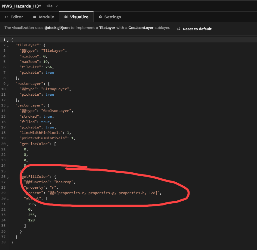
And now our Hazard Types correspond to colors.

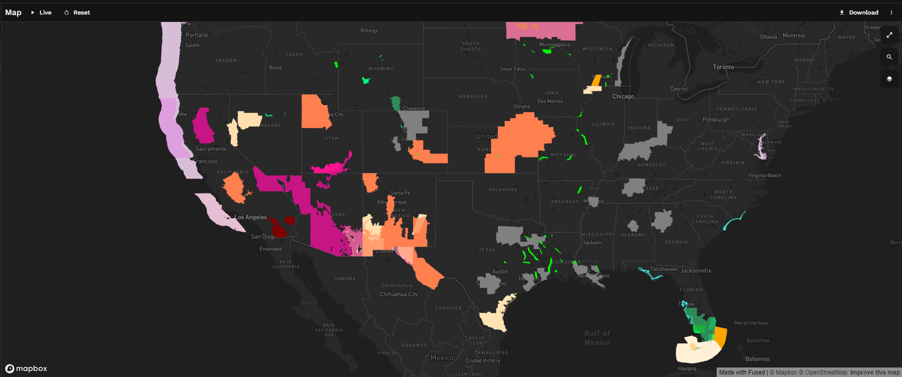
This simple UDF is now complete.

Using it

The beauty of using this framework is we're able fetch one or many datasets from a variety of sources, apply some enrichment, and then save all of that logic for later use by other applications

Now we've fetched raw data (check). Applied some (mild) enrichment. And saved our logic for later use.

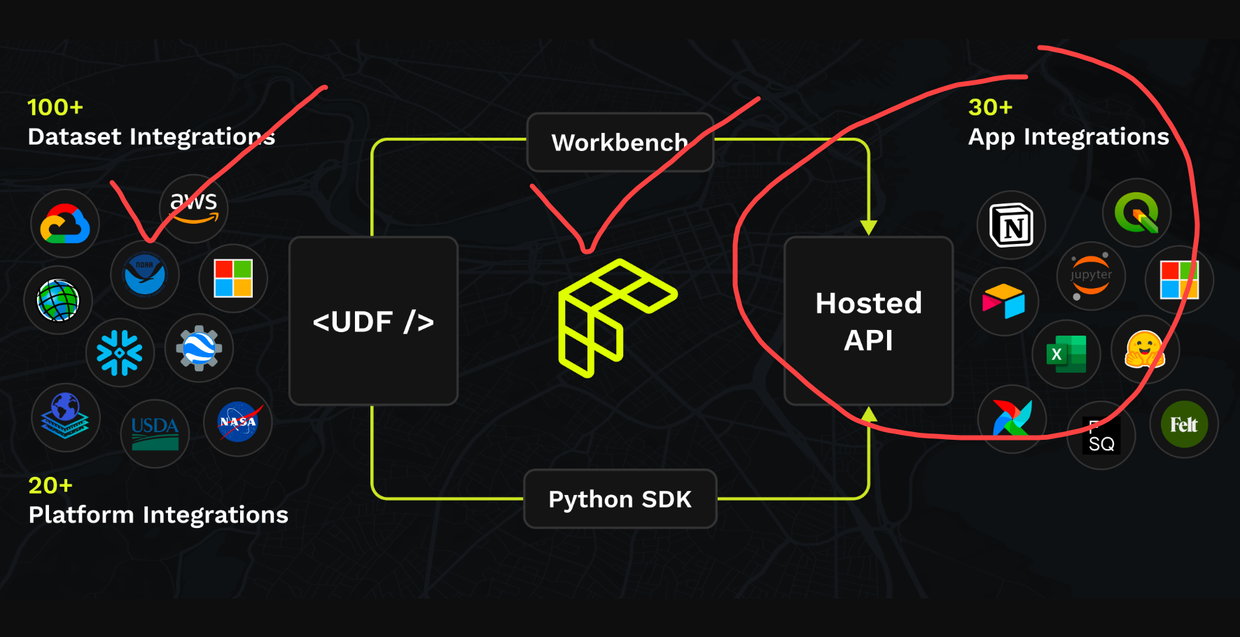
Time to fetch our work with another application. Here's an example use case.

Identify hospitals with hazard risk

Say you're someone with an interest in emergency management.

You'd likely also have an interest in hazards as they're often precursor signal to emergencies.

One consideration in your preparedness planning and response - hospitals.

They're the primary centers for treating injuries & illness. Keeping them operational to serve affected populations during emergencies would be quite important. More specifically, you'd likely be thinking about:

• Ensuring continuity of care
• Resource allocation and planning
• Evacuation and emergency response
• Mitigating facility overload

Being able to quickly identify hospitals with a relatively high probability of hazard risk would be a handy tool to have in your kit.

Let's use our UDF to do that.

First, we'll install and import our libraries.

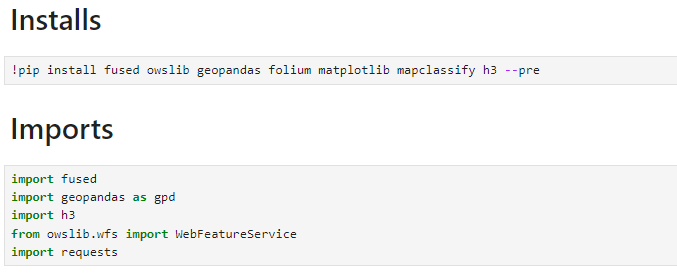
Then we'll call our NWS_Hazards_H3 UDF to fetch current hazards with our desired H3 cell resolution and view them with our colormap.

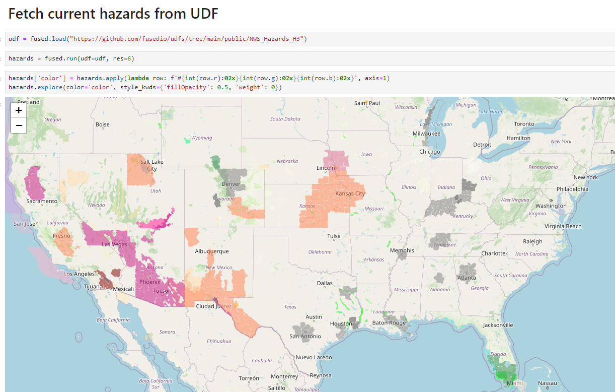
Let's say we only care about the most critical hazard types. Of the three categories Watches, Warnings, and Advisories the group considered the most acute. You may recall:

A warning is issued when a hazardous weather or hydrologic event is occurring, is imminent, or has a very high probability of occurring. A warning is used for conditions posing a threat to life or property.

Let's filter our Hazards gdf to include only Warnings.

(You could alternatively pass specific Hazard Types that are of particular interest to you)

Now let's fetch hospitals.

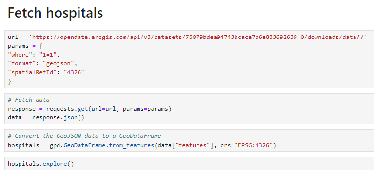
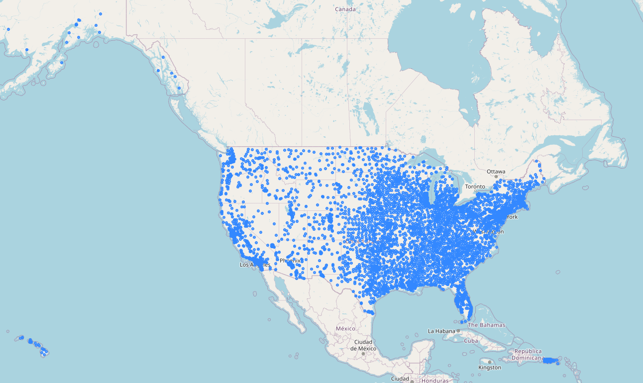
Lot's of em. (8,013 as of today). Let's isolate them to those at increased risk.

We'll start by creating a buffer zone around hospitals for a couple reasons:

1. Hazard zones move over time. Better to cast a wider net in case your hospital is near, but not within, a hazard zone yet.
2. Even if a hospital never crosses paths with a hazard zone, if one is nearby then that community may very well seek treatment at that hospital.

We'll pick a 5 kilometer buffer.

Then we'll join our hospital_buffers gdf to our warnings gdf to select only the areas where hospital buffers intersect with our warning zones.

Then from our joined gdf we'll swap out our geometries to represent the hospital points instead of the buffer zones.

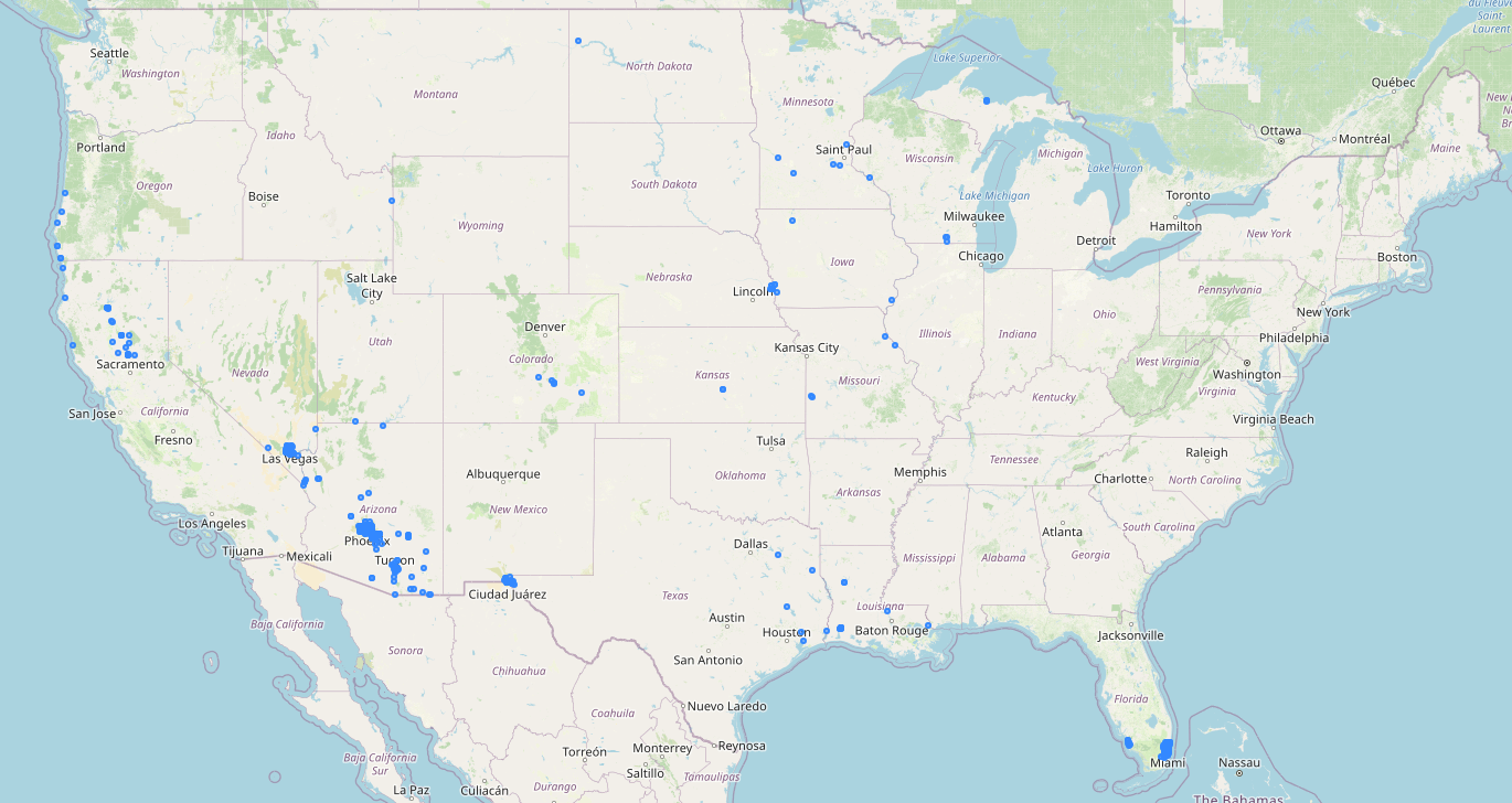
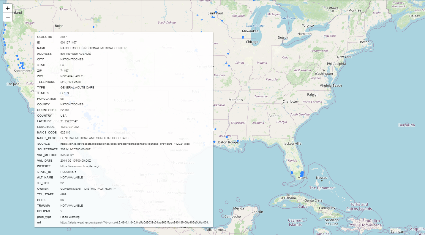
The results is our mapped hospitals_at_risk gdf showing all hospitals that fell within our warnings hazard zones including all hospital attributes plus the applicable hazard type and a link to the hazard alert.

And there you have it.

I'd encourage you to check out Fused and H3. They're powerful tools and I look forward to using them more. And if you have some cool ideas for other use cases please feel free to give me a shout.

And if you want to use this UDF - you can fetch it here:

udfs/public/NWS_Hazards_H3 at main · fusedio/udfs

Public Fused UDFs. Build any scale workflows with the Fused Python SDK and Workbench webapp, and integrate them into your stack with the Fused Hosted API. - fusedio/udfs

GitHubfusedio

Cheers.