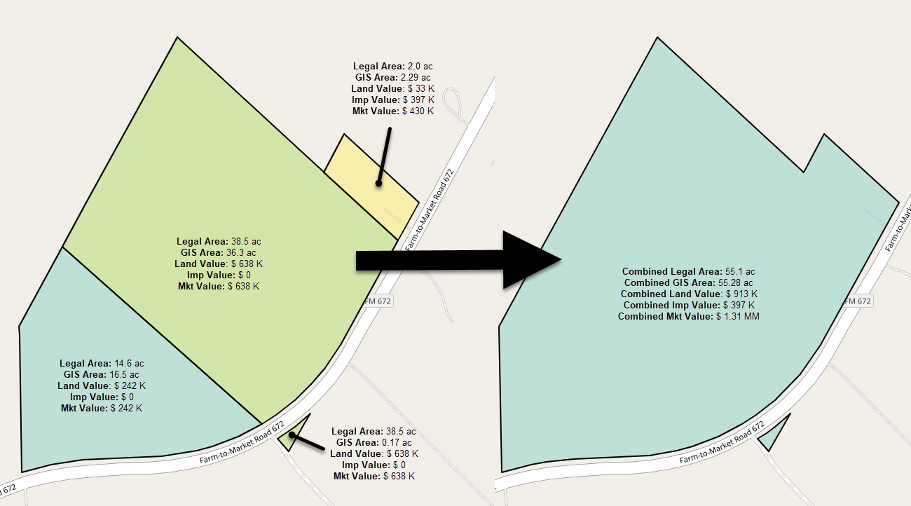
Those that deal in Texas land (especially 'bigger' land) would agree that very often a landowner's property is not neatly packaged into a single legally described parcel. Often, that piece of land is represented by two, three or ten distinct parcels.

Many times those parcels are contiguous (they share a common geographic border, or said otherwise - they touch). Other times they're effectively the same 'property' - but perhaps not actually contiguous. A good example of this could be a ranch that spans both sides of a public access road.

Both of these scenarios can pose a challenge for those looking for land of a particular size (especially when looking for land above a minimum acreage).

Here's a randomly selected example from Caldwell County.:

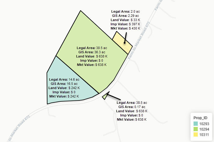
Here we have:

• 4 geographic polygons representing properties in Dale, TX all owned by the same family
• These four polygons are packaged into 3 legally described parcels (10293, 10294, and 10311)
• One parcel (10294 in green) is actually two noncontiguous polygons (separated by a road and right-of-way)
• The other polygons are contiguous
• One parcel (10311) was purchased by just the husband, whereas the others have both the husband and wife noted as owners
• All of the parcels share the same mailing address
• The total legal area here sums to 55.1 acres and total GIS area sums to 55.28 acres.

Now what if I was searching for land for a project and needed a minimum of 50 acres? Let's pretend that this would be an ideal site for that project.

If I were searching for properties with a legal area or GIS area of ≥ 50 acres I would, unfortunately, miss this property - as each of the individual parcels fall below that threshold.

And that would be a bummer... this being the perfect site and all.

A better way to search

When searching for sites, we commonly look for properties that fall above a minimum acreage or within an acreage range:

"Which parcels have an area greater than or equal to {my minimum acreage threshold}?"

As we saw above, this approach turns a blind eye to a bunch of viable options. A better question to ask ourselves is:

Which combination of (contiguous or nearby) parcels with a high probability of the same ownership fall above {my minimum acreage threshold}?

There are two important components there:

1. Contiguous or nearby
2. A high probability of the same ownership

We'll need to address both to derive much value.

Contiguous or nearby

First, for any given parcel we want to determine which other (neighboring) parcels we need to evaluate to make a judgement on whether or not they share an owner. To do this, we'll use the Python Spatial Analysis Library (libpysal).

On my first iteration here, I treated contiguous and nearby separately. I used the libpysal.weights.Rook class to identify contiguous parcels and then subsequently created a buffer around parcels and performed a simple spatial join between parcels and their buffers to identify those parcels that are spatially close, but not directly contiguous.

But then I discovered the libpysal.weights.fuzzy_contiguity class that effectively accomplishes the same goal right out of the box.

Some notes on fuzzy_contiguity :

On my second iteration I was able to use this, passing the same buffer size, and achieve the same desired results.

We'll start by generating our fuzzy contiguity spatial weights matrix.

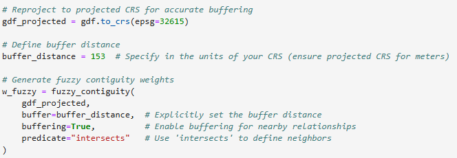
I set a buffer distance of 153 meters, which is just over 500 feet. I believe that should capture most interstate highway right-of-ways and everything smaller.

Here we're capturing all neighbors that touch, contain, or are within 500 feet of the subject parcel.

High probability of shared ownership

We have a few attributes immediately available to us for each parcel that signal ownership:

• The owner's name
• The owner's name in care of
• The mailing address of the owner

As you'll recall above with the Franks' properties above, one of the parcels was in the husbands name only. The others were both husband and wife. If we matched on owner's names alone - we'd be treating those as different properties.

Matching on mailing address helps here. In fact, I think it is likely the better attribute to match on. But there are scenarios where it will fall short too.

For that reason, I decided to consider any match of owner name, owner name in care of, or owner mailing address to qualify as the same ownership.

This is an imperfect solution. But it's a great step in the right direction.

Note for the future - I'd love to be able to graph directorship / membership of Special Purpose Entities and join that to parcel data to see what the real network of ownership of land control looks like.

But for now, we'll stick to our 3 attributes.

We'll construct a network graph (using NetworkX) to model the relationships between parcels based on the fuzzy contiguity weights generated above. We'll filter edges of the graph by verifying that parcels share common ownership attributes:

• OWNER_NAME
• NAME_CARE
• MAIL_ADDR

This filtering step ensures that only parcels with shared ownership characteristics are connected in the graph. The result is a graph that accurately reflects both spatial and ownership relationships.

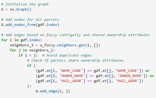
And after our graph is built, we'll segment our commonly-owned parcels into groups using the networkx.connected_components class:

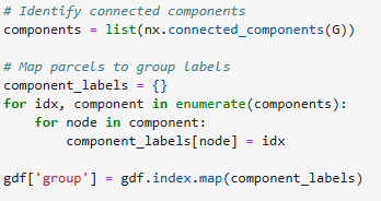
The result is an updated geodataframe that now includes our group field - identifying our contigously(ish) owned parcels. Here are the familiar Franks properties all packaged into group 176:

Dissolving & tidying up the measures

We could stop here with our enriched parcel data, but I think it would be helpful to produce a new dataset that represents each group of contiguously(ish) owned land as it's own unique feature that can be immediately queried.

To do this we'll:

1. Dissolve parcel polygons based on their group
2. Aggregate the parcel dimensions and measures so we can quickly see their total areas and total values.

First we take a special step to handle scenarios where a legally described parcel is represented across more than one polygon. In this case, GIS area should be summed, but all other attributes should be identical - as the'ye tied to the property ID.

Next we'll dissolve our commonly owned land and aggregate area and value measures.

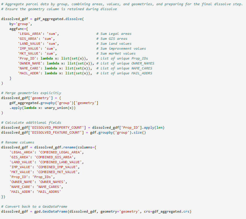
And here's the result for the Franks.

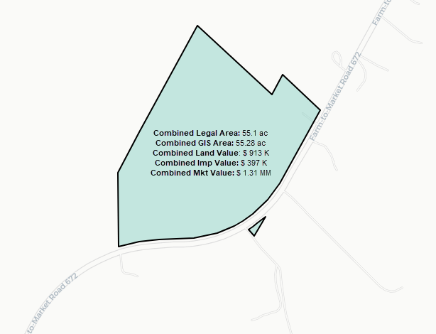
Much easier to query now for my ≥ 50 acre search 😁.

Pretty big impact

Here you can see all of the land parcels (unaltered) for Caldwell County.

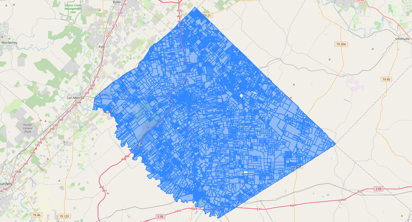
Here's all of the contiguously(ish) owned land comprised of >1 parcel following our work above.

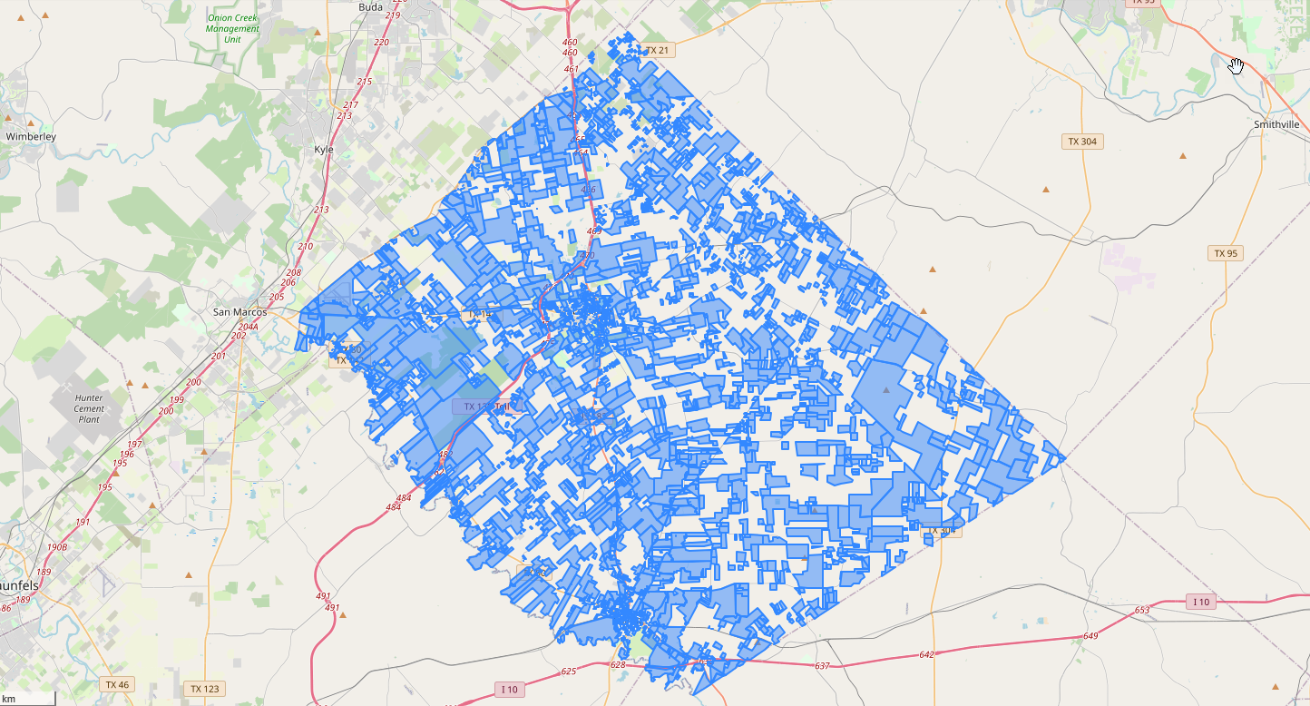
Not too shabby.