You've heard of the poor man's data lake with DuckDB (and Dagster).

(Or maybe you haven't, in which case you should absolutely read (or watch) Pete Hunt and Sandy Ryza's write up on the topic). It's an excellent how-to that will provide you with a low-cost (zero dollar) starting point for building and orchestrating a data lake (or whatever your preferred aquatic data term happens to be).

This write-up is very much in the same spirit. But it's for a specific use case that's a little more niche and it addresses a problem that I'd like to solve immediately.

Namely:

• fetching all different kinds of geospatial data from all different kinds of sources
• performing some transformations (mostly mild)
• co-locating that data in a shared location
• in the same (optimized) format
• such that it's (mostly) accessible by downstream tools (locally and from the web)

Additionally, I wanted a solution that:

• was as low-cost as could be reasonable without hamstringing the goals above
• didn't back me into a vendor corner
• provided me with flexibility

I suspected that Dagster might be the right tool for this, but it'd been over a year since I'd played with it and frankly I was a little intimidated by it. Being new to the geospatial data industry I figured there's probably a tool out there designed specifically to address this obviously common use case. Right?

So I asked my friend Matt Forrest.

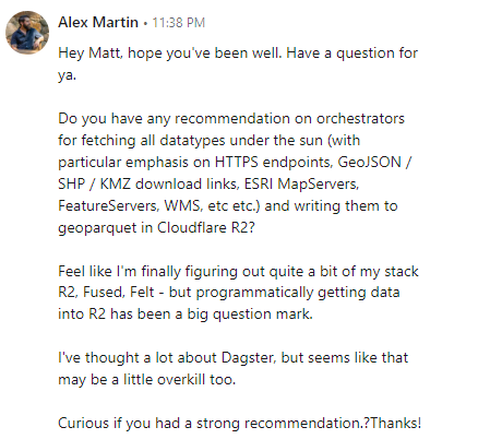
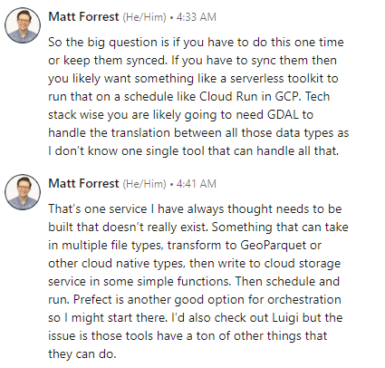
And here we are 😎. Custom solution it is!

(By the way, if you don't already know who Matt is and you're interested in learning anything geospatially related - I highly recommend giving his YouTube channel a watch. There's an absolute wealth of wisdom on there about the most relevant spatial topics).

Scoping our solution

So there's a few questions I needed to answer:

1. What kind of data will I be dealing with?
2. What options do I have for how I fetch that data?
3. Where do I want to store it?
4. How do I want to use it? (Where, how, and with what will I access that data store)?
5. How will I balance convenience vs cost?

And here are my answers...

1. Mostly geospatial data (mostly vector) and your standard tabular / relational data. Some raster, but not much.
2. I will very often be fetching data from ArcGIS endpoints, other APIs, and download links. Perhaps a little web-scraping here and there.
3. Cloudflare R2 and a NAS at my home. The NAS storage is free, but it doesn't cut it if I want to hook other web-apps up to it. R2, from what I understand is a good AWS S3 alternative with no egress fees.
4. Mostly I want to be able to query it with:
   1. Python (Jupyter / Fused)
   2. SQL (DuckDB / MotherDuck)
   3. Custom data apps (Panel, Streamlit, Observable)
   4. Web maps (Felt / Foursquare)
5. Bias towards cost-conscious, serverless, and/or open-source solutions wherever possible. Only choose the paid versions when the relative convenience outweighs the cost.

(Note, we're not building a strictly free solution here - but I do believe this will be a very low relative cost solution for what we gain. Especially considering many of the alternatives).

Why Dagster?

Frankly, it's just such a damn pleasure using the tool. I can't tell you how many times I've been using it, reading their docs, or watching a demo and thought to myself "wow this is great - awesome that they thought of {some feature} and included it out-of-the-box". Some examples.

• Their many integrations with other vendors (like dbt)
• Quick path to unit-testing
• Event logging
• Their visual DAG UI
• Different flavors of triggering workflows
• Partitioning and backfilling
• Tagging, grouping, and customizable metadata
• Dependency declaration

Word of warning: it is not a no-code or low-code solution and there are some nuances that just take some time to learn (or relearn).

Dagster is one of the big names in the data engineering / data orchestration circles. I don't know if they were the first to coin the term "Software Defined Assets (SDAs)" in the context of data engineering, but from my view at least - they certainly seem to be the one's who popularized it.

If you'd like to read up on SDA's I'd recommend starting here.

The product is structured around this core concept and directs you to thinking about the assets that you want to exist and declaring them as python functions rather than the more traditional orchestration way of thinking: do this thing at this time, then do that thing at that time, etc..

The result is you are able to produce chains of assets with overt lineages and clarity around how up-to-date an asset is (or isn't) and why.

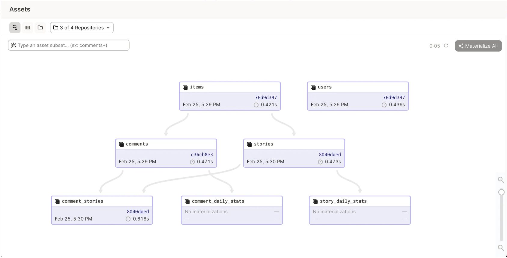
I wound up choosing to go with Dagster over Prefect or Luigi because:

1. I'm familiar with it and really like it
2. It's data asset focus
3. They have self-hosted, hybrid, and fully serverless options (which are all pretty easy to switch too and from as I learn more about my personal convenience-vs-cost thresholds)

I like the idea of being able to use Dagster+ (their paid hosted offering) some of the time if I need an asset refreshed quite regularly or now, but not being backed into it. (Having the ability to trigger workflows locally with no associated compute cost as well).

Why R2?

I mostly covered this already but it's:

• Relatively inexpensive cloud object storage
• Widely accessible
• S3 compatible
• No egress fees

And from my experience so far, very user friendly. I've found that the path to setting up a bucket and getting data in/out is quite a bit clearer than AWS.

(I will also be using my local NAS and DuckDB / MotherDuck some, but for this write-up we'll focus on R2).

Why GeoParquet?

The name is a dead giveaway, but it's the .parquet file format for geospatial vector data.

• It's lighting quick to load into tools like GeoPandas and Lonboard
• Compresses down to much smaller file sizes vs the same dataset in GeoJSON
• Is cloud-optimized
• Coherent and efficient (looking at you shapefiles 🙃)
• It's becoming one of the new standards

Alright. Let's get started.

Building Dagster from a template

Let's start with a fresh repo and virtual environment.

python -m venv .venv
.venv\Scripts\Activate.bat

Now we have a few common options for getting the Dagster raw materials up and running. You can:

1. Create a new project from a Dagster scaffold (default project skeleton). This is the cleanest and most simple approach. Tutorial on that here.
2. You can clone one of Dagster's many use-case specific example projects. This is a great option if you want to explore an existing implementation. Tutorial for this (using their Quickstart example) here.

We'll go with the first.

pip install dagster
dagster project scaffold --name poboy-pipeline-example
cd poboy-pipeline-example
pip install -e ".[dev]"

And now our project skeleton is ready to go.

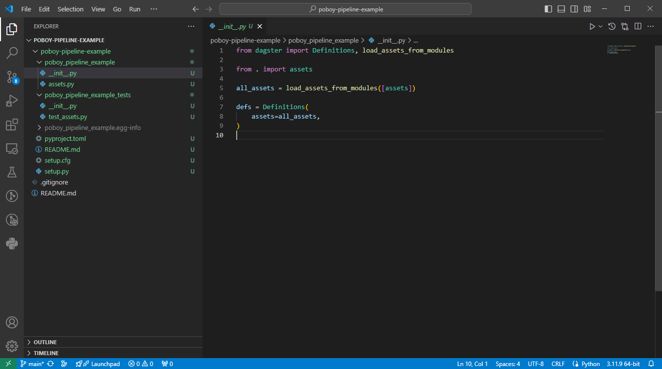
We can now launch the Dagster UI.

dagster dev

Open up your browser and navigate to  http://localhost:3000

Now since we started from the scaffold our project will be pretty bare. (If you're just getting familiar with Dagster try cloning an example - you will be able to see a working pipeline implementation.)

Here's our Assets tab as it stands.

Not much there. Let's remedy that.

Creating our first asset

Now let's create our first software-defined asset so we have something to look at.

You'll recall I listed a handful of geospatial data source types that I want to be able to source from. Many of the raw data sources I fetch are public government-owned datasets. These overwhelmingly live in the ESRI / ArcGIS ecosystem.

As a result of that, one of the most common source types for me is the ArcGIS REST Services FeatureServer. So it only makes sense that this is the first source we implement.

Let's get started with a simple example.

Here's a dataset I find useful.

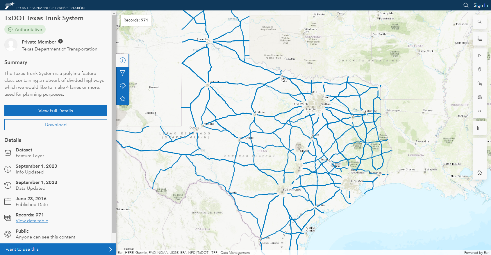
This is the Texas Department of Transportation (TXDoT) Texas Trunk System dataset. Just like the summary says - it's a dataset of the divided highways that they'd like to make 4-lanes wide or more.

Let's fetch the GeoJSON and from that we'll build a GeoPandas GeoDataFrame.

First we'll need to install GeoPandas:

pip install geopandas

This is a good time to mention the setup.py file. Here we can specify new python dependencies like the geopandas library:

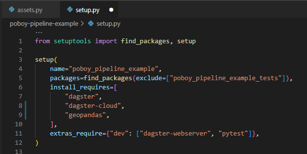
Now let's create that asset.

In our assets.py file we'll import our necessary libraries and we'll create a regular ole python function just like we would anywhere else - with one exception. We'll add the Dagster @asset() decorator above the function.

from dagster import asset
import geopandas as gpd
import requests

@asset()
def texas_trunk_system():
    """ Fetches the TXDoT Texas Trunk System containing a network of divided highways intented to become >= 4 lanes."""
    
    # Define query
    url="https://services.arcgis.com/KTcxiTD9dsQw4r7Z/arcgis/rest/services/TxDOT_Texas_Trunk_System/FeatureServer/0/query"
    params = {
        'where': '1=1',
        'outFields': '*',
        'f': 'geojson',
        }
    
    # Fetch data
    response = requests.get(url, params=params)
    data = response.json()
    
    # Construct geodataframe
    gdf = gpd.GeoDataFrame.from_features(data['features'], crs="EPSG:4326")

    return gdf

Now save your changes. Head back over to your Dagster Dev UI and on the Deployment tab click Reload.

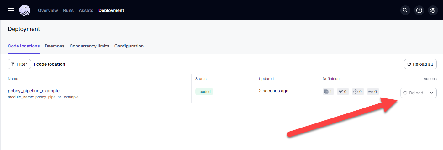
After reloading we can now see our new asset in the Assets tab:

Click on the asset and hit Materialize.

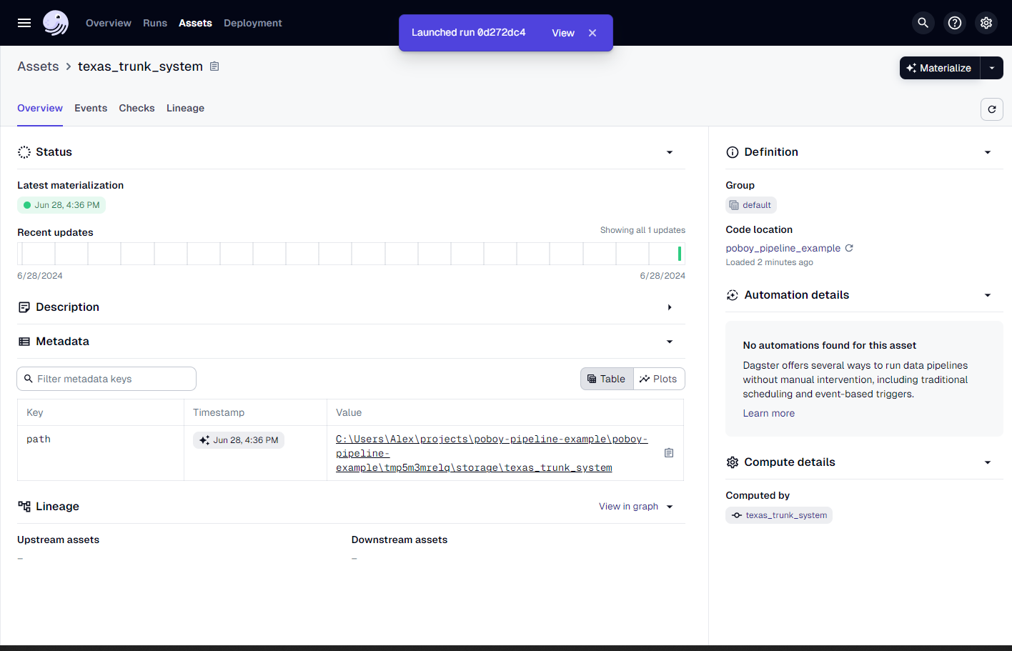
We can click on the launched run and watch the progress as it executes.

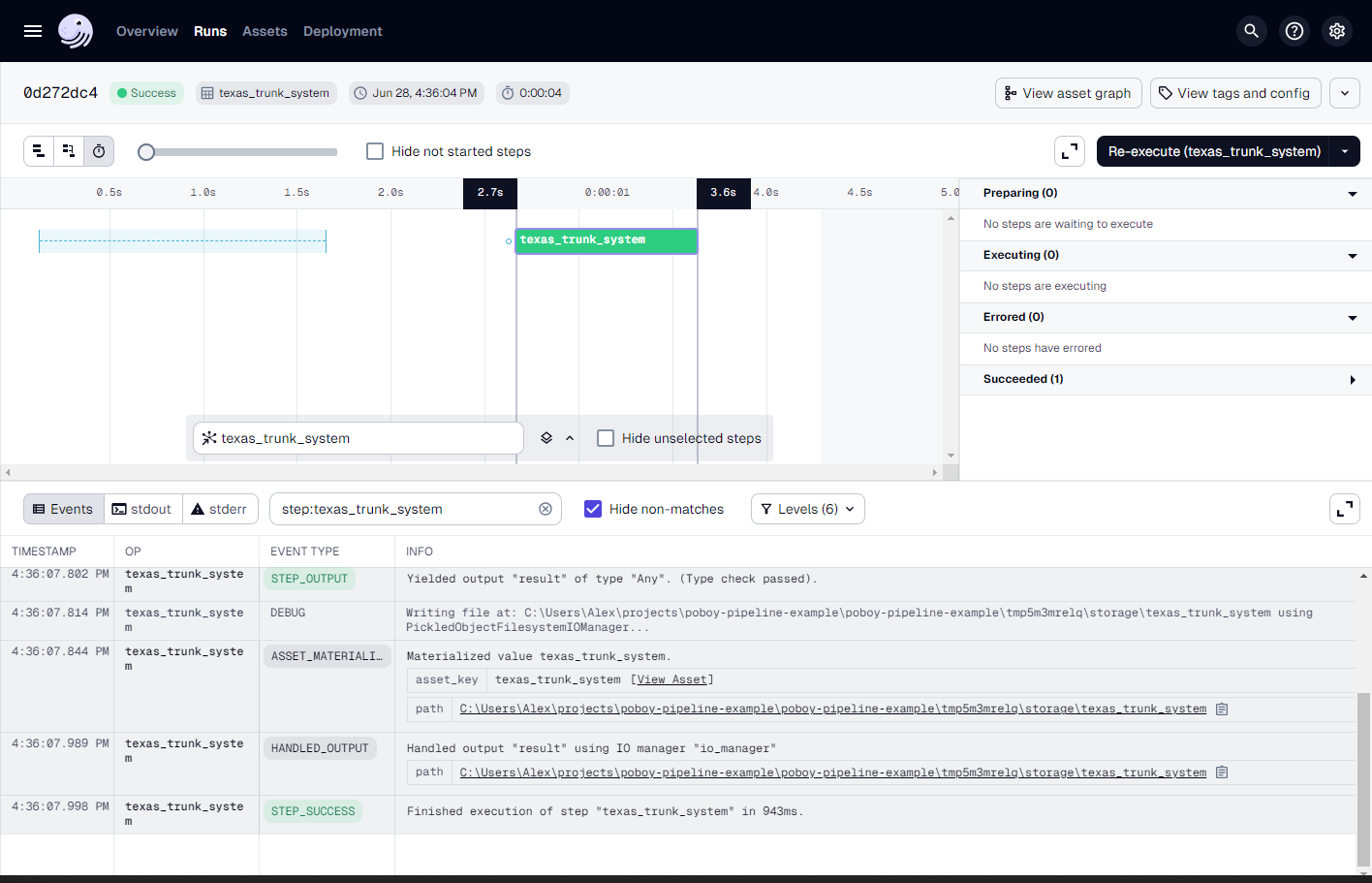
Success!

But there's not a whole lot for us to look at beyond the green event records (which we know means good 😅). By default Dagster uses their FilesystemIOManager to store and retrieve values from pickle files on your local file system. Here we go:

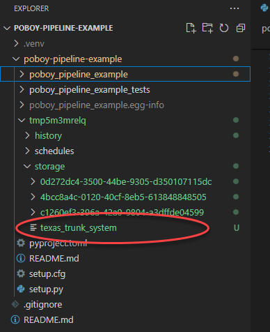
But that's not what we're after. We want to write data to R2 (and down the road we also want to write to a on-prem NAS). Both of these will be very common use cases for me. Almost anything I fetch I'll want to write to one or both of theses locations.

To Resource or to I/O Manage?

One of the beautiful things about about the Software-Defined Asset / User-Defined Function approach to creating data assets (and moving data to and from those assets) is the inherent modularity of it all.

You wrap your business logic in a function and, largely, can restrict the functions code to exactly that - business logic.

The more mundane logic of establishing a session, connecting to a service, paginating API calls, writing data to the right directory, etc. can (and often should) live elsewhere and simply be called by the SDA when needed. This is especially true for code that would otherwise need to be repeated again and again.

Now. I know that I'll be reading and writing to R2 a lot. And I'll be interacting with ArcGIS FeatureServers a lot.

(The nitty-gritty non-business logic to handle those interactions is a prime example of code that should live in some kind of utility class. Not within the asset itself).

Doing so will allow us to:

1. Keep our code modular
2. Make things much easier to read
3. Will drastically reduce the amount of repeat code with inevitable logic variations that introduce risk and accrue technical debt
4. Will provide standardization for how we do {a thing} - so we can expect the same behavior each time.

In the Dagster world - it seems that the two usual suspects for handling this kind of activity are Resources and I/O Managers (which are actually just specialized resources).

So why should I consider using a Resource, you might ask?

What about I/O managers?

Cool! When shouldn't I use an I/O manager?

So what did I choose?

Initially I decided to create a custom IO Manager based on the UPathIOManager class (source linked here). All of the "should" boxes were checked for me but admittedly, one or two of the "shouldn't" boxes were checked too. Looking back, this recommendation from the Dagster I/O managers page was probably the most profound:

As a general rule, if your pipeline becomes more complicated in order to use I/O managers, or you find yourself getting confused when implementing I/O managers, it's likely that you are in a situation where I/O managers are not a good fit. In these cases you should use deps to define dependencies.

(Here's another clear and concise Q&A to consider when you're deciding: "When do I use IO Managers vs a Resource to interact with data?")

I liked the ease that the I/O manager approach provided for passing data and context from one asset downstream to the next. And how it simplified asset definitions.

But ultimately I found that my I/O manager wasn't able to fetch and pass the necessary context with ease to handle some of my quite specific use cases. Ex:

• Sometimes I want to partition data. Often the data I fetch will have semi-random or consistently incomplete temporal partitions
• Sometimes I want full snapshots (but don't want to overwrite old snapshots) and want to pass timestamps and/or run IDs to filenames
• I may want to fetch all or any combination of those

After thoroughly abusing the Dagster @Scout bot in their #ask-ai channel and getting some help in #ask-community, I realized that to get my I/O manager to do what I wanted - I'd have to do some pretty hacky stuff.

Alas, I found my pipeline more complicated and I found myself getting pretty confused.

Resources it was!

Cloudflare R2 resource

Now, let's tackle my most common (and immediately applicable) use case for building a Dagster Resource - interacting with R2.

Here's what I want to do (many times over):

• Write data to specific bucket(s)
• With a specific organization strategy based on an assets metadata (ex. "nesting" files in a particular "directory" structure. Ex: /layer/source/data_category/asset/segmentation_type /segment.filetype
• In specific formats
• Varying somewhat based on environment
• And do all of the above for a bunch of different assets

To start, I want to:

• Write GeoPandas GeoDataframes to GeoParquet in R2
• Read GeoParquet data from R2 and return as a GeoPandas GeoDataframes
• ... and do so for various segmentation strategies (snapshots and partitions) and handle scenarios where data is missing

First, we'll visit our Cloudflare Dash and generate an API token if we don't already have one:

https://dash.cloudflare.com/profile/api-tokens

Then we'll create a .env file within our Dagster project directory to store the necessary variables.

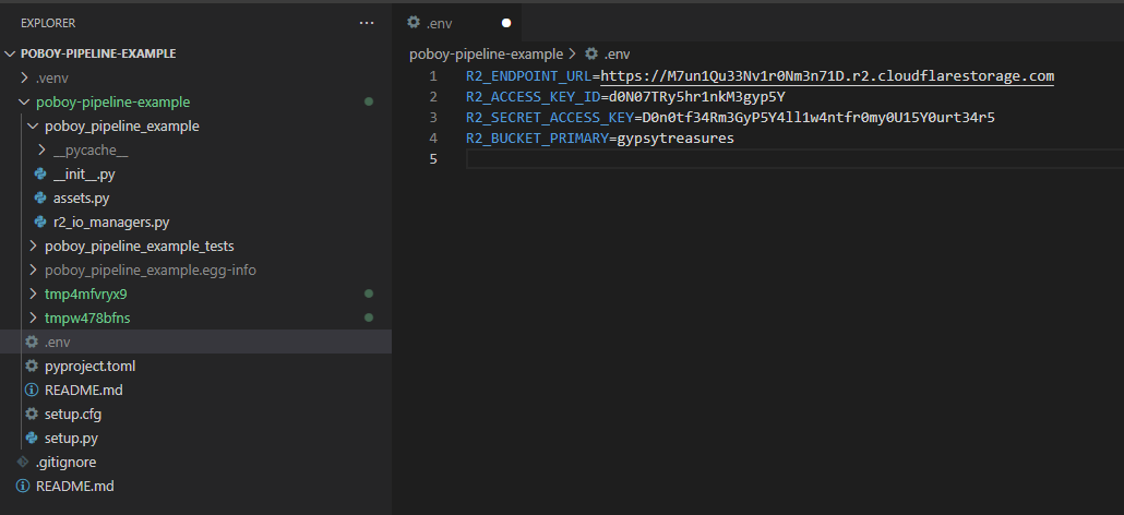
Then we'll create another file within our main project directory resources.py.

NOTE: there are a bunch of ways you can organize your primary Dagster objects (assets, resources, io_managers, schedules, jobs, definitions, etc ). You could:

• Define them all in a single __init__.py file
• Or nest each in it's own file in it's respective directory
• Or do anything in between

I think somewhere in between is the right answer and I have found that starting simple and then increasing the depth of the repo structure as clutter accrues is the best way to keep myself sane 😄.

On to our R2 definition. First things first, we'll create our CloudflareR2DataStore class and declare attributes:

from dagster import ConfigurableResource, AssetExecutionContext, MetadataValue
import requests
import json
import boto3
import io
import geopandas as gpd
import pandas as pd
from upath import UPath
from pydantic import PrivateAttr
from datetime import datetime

class CloudflareR2DataStore(ConfigurableResource):
    """
    Custom resource for handling GeoParquet files stored in Cloudflare R2.

    This manager supports various partition types and handles cases where data might be missing.

    Attributes:
        endpoint_url (str): The endpoint URL for Cloudflare R2.
        access_key_id (str): The access key ID for authentication.
        secret_access_key (str): The secret access key for authentication.
        bucket_name (str): The name of the bucket to use.
    """
    endpoint_url: str
    access_key_id: str
    secret_access_key: str
    bucket_name: str

    _base_path: UPath = PrivateAttr()
    _r2: boto3.client = PrivateAttr()

Next we'll add a setup_for_execution method to initialize our Cloudflare boto3 client using our associated environment variables and we'll define our base path for R2 interactions.

    def setup_for_execution(self, context):
        """
        Initialize the Cloudflare R2 client for execution.

        Args:
            context: The execution context.
        """
        self._base_path = UPath(f"https://{self.endpoint_url}/{self.bucket_name}")
        self._r2 = boto3.client(
            's3',
            aws_access_key_id=self.access_key_id,
            aws_secret_access_key=self.secret_access_key,
            endpoint_url=self.endpoint_url
        )
        context.log.info(f"Initialized Cloudflare R2 client for bucket: {self.bucket_name}")

Next we'll define a method _get_r2_key to generate the unique keys for storing or retrieving R2 objects. This is built to handle both partitioned and un-partitioned assets by constructing the key based on metadata and either partition information or snapshot timestamps. The big point of this is to programmatically organize my data based on declared asset metadata.

At the moment, I've settled on the below logic for partitioned vs unpartitioned assets:

Partitioned:

r2_key = f'{layer}/{source}/{data_category}/{asset_name}/{segmentation}/{partition_key}.geoparquet'

Unpartitioned:

r2_key = f'{layer}/{source}/{data_category}/{asset_name}/{segmentation}/snapshot={timestamp}.geoparquet'

This may be too many forward slashes and I may revise it down the road. But for now it's okay.

Here's the full method definition.

    def _get_r2_key(self, context: AssetExecutionContext) -> str:
        """
        Generate the R2 key for storing or retrieving an object.

        This method handles both partitioned and non-partitioned assets.

        Args:
            context (AssetExecutionContext): The context for the operation.

        Returns:
            str: The generated R2 key.
        """
        asset_key = context.asset_key
        metadata = context.assets_def.metadata_by_key[asset_key]
        layer = metadata.get("layer", "fallback_layer")
        source = metadata.get("source", "fallback_source")
        data_category = metadata.get("data_category", "fallback_category")
        asset_name = asset_key.path[-1]
        segmentation = metadata.get("segmentation", "fallback_segmentation")
        
        if context.has_partition_key:
            partition_key = context.partition_key
            r2_key = f'{layer}/{source}/{data_category}/{asset_name}/{segmentation}/{partition_key}.geoparquet'
        else:
            timestamp = datetime.now().isoformat()
            r2_key = f'{layer}/{source}/{data_category}/{asset_name}/{segmentation}/snapshot={timestamp}.geoparquet'
        
        return r2_key

Next we'll define how we want to write fetched data to R2 with the write_gpq method. This converts the GeoDataFrame to a GeoParquet file, uploads it to R2, and logs metadata such as write location, file size, and number of records.

    def write_gpq(self, context: AssetExecutionContext, gdf: gpd.GeoDataFrame):
        """
        Save a GeoDataFrame to Cloudflare R2.

        Args:
            context (AssetExecutionContext): The context for the operation.
            gdf (gpd.GeoDataFrame): The GeoDataFrame to save.
        """
        if gdf is None or gdf.empty:
            context.log.info("No data available for this partition. Skipping write operation.")
            return

        try:
            object_key = self._get_r2_key(context)
            full_path = self._base_path / object_key
            context.log.info(f"Preparing to upload to path: {full_path}")

            buffer = io.BytesIO()
            gdf.to_parquet(buffer, engine='pyarrow', index=False, compression='snappy')
            buffer.seek(0)
            file_size = buffer.getbuffer().nbytes

            self._r2.upload_fileobj(buffer, self.bucket_name, object_key)
            context.log.info(f"Uploaded file to {full_path}")

            metadata = {
                "r2_write_location": MetadataValue.text(str(full_path)),
                "r2_file_size_written": MetadataValue.text(format_size(file_size)),
                "r2_num_records_written": MetadataValue.int(len(gdf)),
            }

            context.add_output_metadata(metadata)

        except Exception as e:
            context.log.error(f"Failed to upload file: {e}")
            raise

Next we have 3 flavors of read methods:

1. read_gpq_single_key: Read a single R2 object (aka a single file) by explicitly specifying it's key.
2. read_gpq_all_partitions: Read in (and combine) all partitions associated with a given key pattern. There's no such thing as a "folder" in R2, but think of this like reading in every file from a specified folder. Say you have daily orders data that landed here. Using this method you'd fetch all orders across all days.
3. read_gpq_latest_snapshot: Read in the most recent snapshot of an asset, given a specific key pattern. Same "folder" concept as above, but in this example we have multiple snapshots of full datasets. Say you store some data here that's sporadically updated. You have a snapshot from last November, this February and this March. This method would fetch the March file.

    def read_gpq_single_key(self, context: AssetExecutionContext, key: str) -> gpd.GeoDataFrame:
        """
        Load a GeoDataFrame from Cloudflare R2 using a specific key.

        Args:
            context (AssetExecutionContext): The context for the operation.
            key (str): The specific R2 key to load the object from.

        Returns:
            gpd.GeoDataFrame: The loaded GeoDataFrame, or an empty GeoDataFrame if no data is available.
        """
        try:
            full_path = self._base_path / key
            context.log.info(f"Attempting to download from path: {full_path}")

            buffer = io.BytesIO()
            self._r2.download_fileobj(self.bucket_name, key, buffer)
            buffer.seek(0)
            file_size = buffer.getbuffer().nbytes

            gdf = gpd.read_parquet(buffer)
            context.log.info(f"Successfully downloaded file from {full_path}")

            metadata = {
                "r2_read_location": MetadataValue.text(str(full_path)),
                "r2_file_size_read": MetadataValue.text(format_size(file_size)),
                "r2_num_records_read": MetadataValue.int(len(gdf)),
                "r2_columns_read": MetadataValue.json(list(gdf.columns)),
                "r2_object_preview": MetadataValue.md(self._get_head_preview(gdf)),
            }

            context.add_output_metadata(metadata)
            return gdf
        except Exception as e:
            context.log.error(f"Failed to download file: {e}")
            raise

    def read_gpq_all_partitions(self, context: AssetExecutionContext, key_pattern: str) -> gpd.GeoDataFrame:
        """
        Load a GeoDataFrame from Cloudflare R2 for all partitions matching a key pattern.

        Args:
            context (AssetExecutionContext): The context for the operation.
            key_pattern (str): The key pattern to match partitions.

        Returns:
            gpd.GeoDataFrame: The combined GeoDataFrame from all partitions.
        """
        try:
            paginator = self._r2.get_paginator('list_objects_v2')
            pages = paginator.paginate(Bucket=self.bucket_name, Prefix=key_pattern)

            all_gdfs = []
            total_size = 0
            total_records = 0

            for page in pages:
                if 'Contents' in page:
                    for obj in page['Contents']:
                        key = obj['Key']
                        if key.endswith('.geoparquet'):
                            gdf = self.read_gpq_single_key(context, key)
                            if not gdf.empty:
                                all_gdfs.append(gdf)
                                total_size += obj['Size']
                                total_records += len(gdf)

            if not all_gdfs:
                context.log.warning(f"No data found for key pattern: {key_pattern}")
                return gpd.GeoDataFrame()

            combined_gdf = pd.concat(all_gdfs, ignore_index=True)
            context.log.info(f"Combined GeoDataFrame with {len(combined_gdf)} total records")

            metadata = {
                "r2_key_pattern": MetadataValue.text(key_pattern),
                "r2_read_location": MetadataValue.text(str(self._base_path / key_pattern)),
                "r2_file_size_read": MetadataValue.text(format_size(total_size)),
                "r2_num_records_read": MetadataValue.int(total_records),
                "r2_columns_read": MetadataValue.json(list(combined_gdf.columns)),
                "r2_object_preview": MetadataValue.md(self._get_head_preview(combined_gdf)),
            }

            context.add_output_metadata(metadata)
            return combined_gdf
        except Exception as e:
            context.log.error(f"Failed to read all partitions: {e}")
            raise
        
    def read_gpq_latest_snapshot(self, context: AssetExecutionContext, key_pattern: str) -> gpd.GeoDataFrame:
        """
        Load the latest snapshot GeoDataFrame from Cloudflare R2 based on a key pattern.

        Args:
            context (AssetExecutionContext): The context for the operation.
            key_pattern (str): The key pattern to match snapshots.

        Returns:
            gpd.GeoDataFrame: The latest snapshot GeoDataFrame.
        """
        try:
            paginator = self._r2.get_paginator('list_objects_v2')
            pages = paginator.paginate(Bucket=self.bucket_name, Prefix=key_pattern)

            latest_key = None
            latest_timestamp = None

            for page in pages:
                if 'Contents' in page:
                    for obj in page['Contents']:
                        key = obj['Key']
                        if key.endswith('.geoparquet'):
                            # Extract timestamp from the key
                            timestamp_str = key.split('snapshot=')[-1].replace('.geoparquet', '')
                            timestamp = datetime.fromisoformat(timestamp_str)
                            if latest_timestamp is None or timestamp > latest_timestamp:
                                latest_timestamp = timestamp
                                latest_key = key

            if latest_key is None:
                context.log.warning(f"No snapshots found for key pattern: {key_pattern}")
                return gpd.GeoDataFrame()

            gdf = self.read_gpq_single_key(context, latest_key)
            context.log.info(f"Loaded latest snapshot from {latest_key}")

            metadata = {
                "r2_key_pattern": MetadataValue.text(key_pattern),
                "r2_read_location": MetadataValue.text(str(self._base_path / latest_key)),
                "r2_file_size_read": MetadataValue.text(format_size(obj['Size'])),
                "r2_num_records_read": MetadataValue.int(len(gdf)),
                "r2_columns_read": MetadataValue.json(list(gdf.columns)),
                "r2_object_preview": MetadataValue.md(self._get_head_preview(gdf)),
            }

            context.add_output_metadata(metadata)
            return gdf
        except Exception as e:
            context.log.error(f"Failed to read latest snapshot: {e}")
            raise

Annnd lastly we have a couple helper functions to create easier to read previews of datasets and file size metadata:

def format_size(size_bytes):
    return f"{size_bytes / (1024 * 1024):.2f} MB"

    def _get_head_preview(self, gdf: gpd.GeoDataFrame, n: int = 5) -> str:
        """
        Generate a preview of the GeoDataFrame, excluding the 'geometry' column if it exists.

        Args:
            gdf (gpd.GeoDataFrame): The GeoDataFrame to generate a preview for.
            n (int): The number of rows to include in the preview.

        Returns:
            str: The markdown representation of the preview.
        """
        preview_df = gdf.head(n).copy()
        if 'geometry' in preview_df.columns:
            preview_df = preview_df.drop(columns=['geometry'])
        return preview_df.to_markdown()

Hits save.

We've now addressed how we want to interact with spatial data within our environment GeoDataFrame ↔ R2 GeoParquet.

This is a big piece of the puzzle and will provide uniformity and efficiency to our data lake.

But it doesn't address the variable landscape of how our source data exists externally out in the wild. That's the other half of the challenge we're solving.

Spatial data in the wild

The impetus for this whole project was to find an answer to the question:

How do I get their data (in all of it's forms) into my storage solution? (With uniformity and efficiency)

Which begs the question:

Well, how do they have their data?

The answer is: a bunch of ways. Here are what I've found to be the most common.

• ArcGIS REST FeatureServer
• ArcGIS REST MapServer
• ArcGIS Web Feature Service (WFS)
• Shapefiles
• GeoJSON
• KMZ / KML

I expect this list to grow over time and I intend to address them all.

But. At this moment - I've already typed 4,462 words. So for the sake of sparing your eyes and my finger tips we'll restrict this write up to addressing only one external source - FeatureServers (which are very common when dealing with government data sources like TXDoT).

Handling common source systems w/ Dagster resources

Again my intent here is to accomplish two things:

1. Keep our Dagster assets, to the greatest extent possible, clean and focused on the business logic of the asset.
2. For generalized and frequently repeated tasks, modularize the logic to accomplish those tasks. This way we can build them once and call them in different places with ease.

This will make developing new assets easier and faster with less repeat code.

We'll be interacting with FeatureServers (owned by many different entities) a lot. Behind each of those FeatureServers will be novel data sets. We want our assets to focus on the nuances of interacting with those data sets. To handle the nuances of interacting with the FeatureServer middle-man, we'll use a Dagster resource.

Let's build a resource to handle our ArcGIS FeatureServers interactions.

We'll start by creating a new class in our resources.py file called ArcGISFeatureServerResource which will inherit the the Dagster base class ConfigurableResource (documentation on that here).

Within that class, we'll create a fetch_data method that...fetches our data.

You saw with our texas_trunk_system asset above that fortunately interacting with Feature Servers is pretty simple. You define the endpoint url and query parameters. You then use those to make an API call with the requests library. And after that you use the fetched features to build a geodataframe.

There are a few things we can do to make that process a little more robust. For example we'll:

1. Obfuscate all the transactional logic from the asset author. All they need to think about is the endpoint, their query, and any transformations.
2. Make sure that the endpoint supports GeoJSON as an acceptable format to return.
3. If you've defined a maxRecordCount parameter, then paginate your API calls if necessary. Not infrequently these FeatureServers have maximum record counts of 2000 or less for a given call. We'll need to be able to handle scenarios where there are > 2000 features on the other side of the API and we want to fetch them all.
4. Handle common exceptions, log progress & issues, and report metadata back to the Dagster UI
5. Build and return a GeoPandas GeoDataFrame with your desired coordinate reference system
6. And if no features are available, return an empty GeoDataFrame

Here's the meat and potatoes of our ArcGISFeatureServerResource class:

class ArcGISFeatureServerResource(ConfigurableResource):
    """
    Resource for querying an ArcGIS FeatureServer and returning data as a GeoDataFrame.
    """

    def fetch_data(self, url: str, params: dict, crs: str = 'EPSG:4326', context=None) -> gpd.GeoDataFrame:
        """
        Query an ArcGIS FeatureServer and return a GeoDataFrame with the specified CRS.

        Args:
        - url (str): The base URL of the FeatureServer endpoint.
        - params (dict): A dictionary of parameters to include in the query.
        - crs (str): The coordinate reference system to set for the GeoDataFrame (default: 'EPSG:4326').
        - context: The Dagster execution context (optional).

        Returns:
        - GeoDataFrame: A GeoDataFrame containing the features retrieved from the FeatureServer.
        """
        all_features = []
        params = params.copy()  # Avoid modifying the original params dictionary
        params['f'] = 'geojson'  # Ensure the response format is GeoJSON
        params['resultOffset'] = 0  # Start from the first record

        max_record_count = params.get('maxRecordCount', None)
        
        api_response = None
        
        while True:
            try:
                response = requests.get(url, params=params)
                response.raise_for_status()
                
                if api_response is None:
                    api_response = f"<Response [{response.status_code}]>"  # Store the response code

                data = response.json()

                if 'error' in data:
                    error_message = f"Error querying FeatureServer: {data['error']}"
                    if context:
                        context.log.error(error_message)
                    else:
                        print(error_message)
                    return gpd.GeoDataFrame()  # Return empty GeoDataFrame

                # Check if 'f' = 'geojson' is not supported
                if 'type' not in data or data['type'] != 'FeatureCollection':
                    error_message = "The server did not return GeoJSON data. Ensure the server supports GeoJSON format."
                    if context:
                        context.log.error(error_message)
                    else:
                        print(error_message)
                    return gpd.GeoDataFrame()  # Return empty GeoDataFrame

                features = data.get('features', [])
                all_features.extend(features)

                if max_record_count and len(features) < max_record_count:
                    break  # No more features to fetch

                # Update the resultOffset for the next iteration
                params['resultOffset'] += max_record_count if max_record_count else len(features)

                # If there are no more features, break the loop
                if not features:
                    break

            except requests.exceptions.RequestException as e:
                error_message = f"Request failed: {e}"
                if context:
                    context.log.error(error_message)
                else:
                    print(error_message)
                return gpd.GeoDataFrame()  # Return empty GeoDataFrame on error
            except json.JSONDecodeError:
                error_message = "Failed to decode JSON response."
                if context:
                    context.log.error(error_message)
                else:
                    print(error_message)
                return gpd.GeoDataFrame()  # Return empty GeoDataFrame on error

        # Convert all collected features to a GeoDataFrame
        if not all_features:
            return gpd.GeoDataFrame()  # Return empty GeoDataFrame if no features found

        gdf = gpd.GeoDataFrame.from_features(all_features, crs=crs)
        
        if context:
            context.log.info(f"Retrieved GeoDataFrame with {len(gdf)} features.")
        
            # Add metadata
            metadata = {
                "api_endpoint_url": MetadataValue.text(url),
                "api_query_params": MetadataValue.json(params),
                "api_response": MetadataValue.text(api_response),
                "api_num_features": MetadataValue.int(len(gdf)),
                "api_features_preview": MetadataValue.md(self._get_features_preview(gdf)),
                "api_columns": MetadataValue.json(list(gdf.columns))
            }
            context.add_output_metadata(metadata)
        
        return gdf

    def _get_features_preview(self, gdf: gpd.GeoDataFrame, n: int = 5) -> str:
        """
        Generate a preview of the GeoDataFrame, excluding the 'geometry' column if it exists.

        Args:
            gdf (gpd.GeoDataFrame): The GeoDataFrame to generate a preview for.
            n (int): The number of rows to include in the preview.

        Returns:
            str: The markdown representation of the preview.
        """
        preview_df = gdf.head(n).copy()
        if 'geometry' in preview_df.columns:
            preview_df = preview_df.drop(columns=['geometry'])
        return preview_df.to_markdown()

This resource will provide us with a nice standardized way to interact with a seemingly never-ending list of FeatureServers.

Implementing our new resources

We've now created two fancy new resources that will help us interact with our stuff (R2) and their stuff (FeatureServers).

In order to use them we need to let the rest of Dagster know about it.

We'll start by adding our new resources to our defs Definition in our __init__.py file.

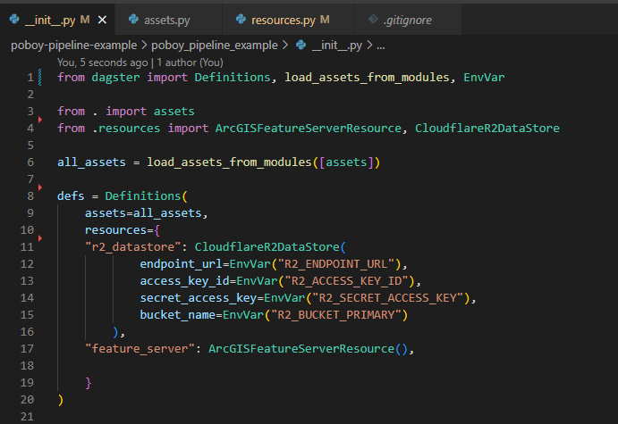
Here we're importing our new resources then we're defining instances of them. In the case of our r2_datastore we're fetching the necessary environment variables to configure our boto3 r2 client.

Great.

Now let's tell our texas_trunk_system asset about them. Here's our updated definition:

@asset(
    group_name='raw_data',
    metadata={"layer": "landing", "source": "txdot", "data_category": "vector", "segmentation": "snapshots"},
    )
def texas_trunk_system(context: AssetExecutionContext, feature_server: ArcGISFeatureServerResource, r2_datastore: CloudflareR2DataStore):
    """ Fetches the TXDoT Texas Trunk System containing a network of divided highways intented to become >= 4 lanes."""
    
    # Define query
    url="https://services.arcgis.com/KTcxiTD9dsQw4r7Z/arcgis/rest/services/TxDOT_Texas_Trunk_System/FeatureServer/0/query"
    params = {
        'where': '1=1',
        'outFields': '*',
        'f': 'geojson',
        }
    
    # Fetch data and return geodataframe
    gdf = feature_server.fetch_data(url=url, params=params, context=context)

    # Write the GeoDataFrame to R2
    r2_datastore.write_gpq(context, gdf)

You'll notice a few things are still the same:

1. We're still defining our endpoint url (business logic)
2. We're still defining our query parameters (business logic)

But you'll also notice a few things different:

1. We've added our metadata and a group name to our asset definition. This will direct the output of our asset to the right location in R2 and help us keep things organized in the Dagster UI, resp.
2. We're passing our resource instances into the asset function
3. We're fetching data from the TXDoT FeatureServer and generating a GeoDataFrame by passing our our business logic to the feature_server.fetch_data() method.
4. We're writing the results of our GeoDataFrame to .geoparquet in R2 by calling the r2_datastore.write_gpq() method.

Shall we hit run and see what happens?

Writing to R2

Hit save on everything in VSCode.

In the Dagster Dev UI navigate back to your Deployment tab and hit Reload. Head over to your Assets tab again and materialize the asset.

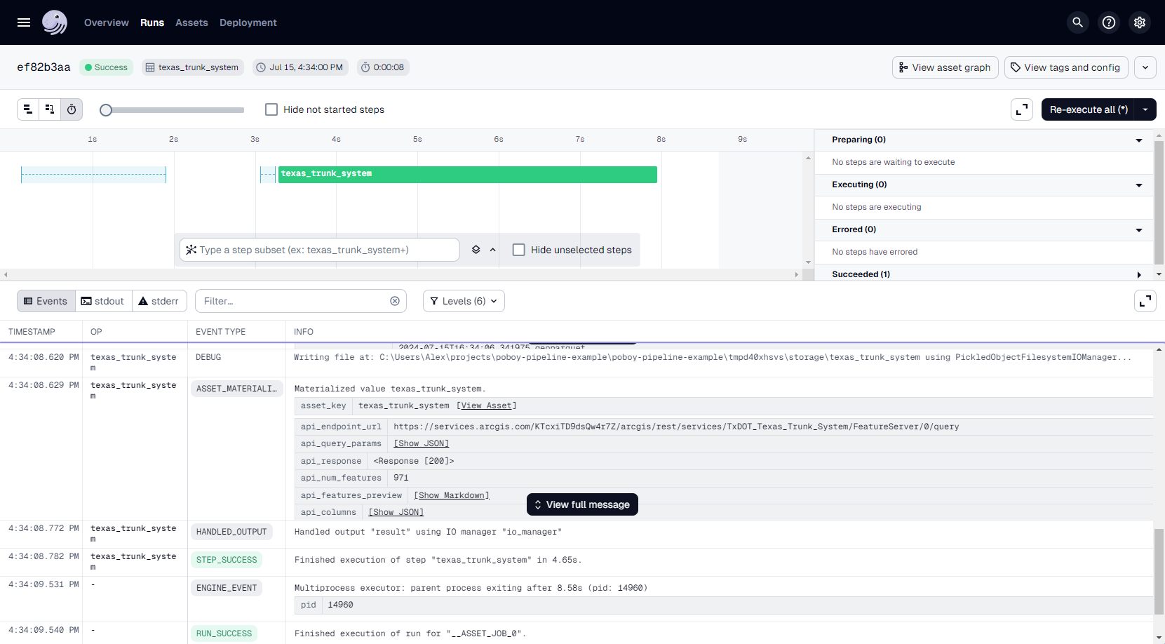
Moment of truth...

Great success.

And we've got some nice metadata in our asset page to go with it.

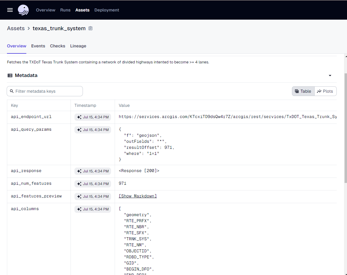
Now for any new spatial assets we create - if we want to write the output to geoparquet in R2 all we have to do is add the appropriate "layer", "source", "data_category", and "segmentation" , metadata arguments to our asset definition, pass our resources to the function, and call our desired method. This'll file it away in the right place.

Since we built it, let's partition it

Now, it'd be perfectly fine to keep our texas_trunk_system asset as a snapshot asset (producing a snapshot of the full dataset at the moment in time the asset is materialized).

It's not a very big asset. It slow changing. And I'd wager it's not updated on a very consistent schedule.

However, it does have a date field. We did build out partitioning functionality. And it wouldn't hurt to see how it changes over time. So let's set it up for partitioning to at the very least just show that it works.

To start we'll define the partition. Dagster has out-of-the-box partition definitions for hourly, daily, weekly, monthly, static, time-window, multi-partitions, and dynamic partitions. Here's the link if you'd like to do some extra reading on it.

They don't have an out of the box yearly partition. With as slow changing as texas_trunk_system is, we'll create a custom yearly partition definition using the time-window partition definition.

from dagster import TimeWindowPartitionsDefinition

# Define yearly partitions starting from 2023
yearly_partitions = TimeWindowPartitionsDefinition(
    cron_schedule="@yearly",  # Run once a year
    start=datetime(2023, 1, 1),  # Start from January 1, 2023
    end_offset=1,  # Include the current year
    fmt="%Y"  # Format partition keys as YYYY
)

We'll then update our asset definition declaring the partitions_def and we'll pass the partition as a filter / argument within our query.

@asset(
    group_name='raw_data',
    metadata={"layer": "landing", "source": "txdot", "data_category": "vector", "segmentation": "partitions"},
    partitions_def=yearly_partitions,
    )
def texas_trunk_system(context: AssetExecutionContext, feature_server: ArcGISFeatureServerResource, r2_datastore: CloudflareR2DataStore):
    """ Fetches the TXDoT Texas Trunk System containing a network of divided highways intented to become >= 4 lanes."""
    
    # Define annual partition key
    year = context.partition_key
    context.log.info(f"Processing partition for year: {year}")
    
    # Define query
    url="https://services.arcgis.com/KTcxiTD9dsQw4r7Z/arcgis/rest/services/TxDOT_Texas_Trunk_System/FeatureServer/0/query"
    params = {
        'where': f"EXTRACT(YEAR FROM EXT_DATE) = {year}",
        'outFields': '*',
        'f': 'geojson',
        }
    
    # Fetch data and return geodataframe
    gdf = feature_server.fetch_data(url=url, params=params, context=context)

    # Write the GeoDataFrame to R2
    r2_datastore.write_gpq(context, gdf)

Above we:

• Define partitions_def=yearly_partitions within the asset decorator
• We update our "segmentation" metadata argument with a "partitions" value
• We fetch the partition key from context year = context.partition_key
• And we update our query to pass the partition filter 'where': f"EXTRACT(YEAR FROM EXT_DATE) = {year}"

The result is our asset now becomes somewhat of a collection of mini-assets, each representing one of our partition values within the range.

We can backfill specific partitions or all partitions within our defined range. NOTE: when you re-run a materialized partition you overwrite the previous results.

Save. Reload. Rematerialize. Boom.

Here is our single partition in all of it's glory.

Not a fantastic showcase of how powerful partitioning can be, but you get the idea. It's very well suited for data with regular updates and/or clear segments.

We now have a modular FeatureServer resource that we can pass to any asset to fetch data from any GeoJSON supported FeatureServer. We can apply additional business logic transformations to the asset if we like. We can write and read both partitioned and unpartitioned assets to and from R2 in GeoParquet.

Mission accomplished.

Adding some downstream assets

Now, I'd say this is realistically the end of this piece of the project. But I want a thumbnail showing a few assets and their dependencies (not just our one texas_trunk_system asset) 😅. So let's add some additional assets, which'll also provide us with the opportunity to see how assets get strung together.

Example analysis

Knowing major transportation thoroughfares pegged for expansion is useful signal for where growth may occur. Our texas_trunk_system asset delivers this.

Another consideration that may suggest how near or far from those thoroughfares a developer may want to be - median household income. And just so we can squeeze a third asset in there, let's fetch county boundary lines as well and filter our results to only a handful of counties of particular interest.

Fetching extra assets

First we'll fetch our counties. We'll source this from TXDoT as well.

@asset(
    group_name='raw_data',
    metadata={"layer": "landing", "source": "txdot", "data_category": "vector", "segmentation": "full_snapshots"},
)
def texas_county_boundaries(context: AssetExecutionContext, feature_server: ArcGISFeatureServerResource, r2_datastore: CloudflareR2DataStore):
    """Fetches the TXDoT polygon layer of the 254 Texas counties"""
    
    # Define query
    url = "https://services.arcgis.com/KTcxiTD9dsQw4r7Z/arcgis/rest/services/Texas_County_Boundaries/FeatureServer/0/query?"
    params = {
        'where': '1=1',
        'outFields': '*',
        'f': 'geojson',
    }
    
    # Fetch data
    gdf = feature_server.fetch_data(url=url, params=params, context=context)
    
    # Write the GeoDataFrame to R2
    r2_datastore.write_gpq(context, gdf)
    
    return gdf

Next, we'll fetch median household income from the Census Bureau's American Community Survey (ACS) from 2018 - 2022. This is a big dataset that offers 3 different layers for metric reporting: state, county, and census tract. We want the finest grain, so we'll select the census tract option.

Since this dataset is so big (and we only care about Texas for this project) we'll filter to only Texas "where": "State='Texas'".

Here's how we do it.

@asset(
    group_name='raw_data',
    metadata={"layer": "landing", "source": "census_bureau", "data_category": "vector", "segmentation": "full_snapshots"},
)
def tx_med_household_income(context: AssetExecutionContext, feature_server: ArcGISFeatureServerResource, r2_datastore: CloudflareR2DataStore):
    """Fetches American Community Survey (ACS) median household income by census tract in Texas."""
    
    # Define query
    url="https://services.arcgis.com/P3ePLMYs2RVChkJx/ArcGIS/rest/services/ACS_Median_Income_by_Race_and_Age_Selp_Emp_Boundaries/FeatureServer/2/query?"
    params = {
        "where": "State='Texas'",
        "outFields": "*",
        "f": "geojson",
        "returnGeometry": "true", 
    }
    
    # Fetch data
    gdf = feature_server.fetch_data(url=url, params=params, context=context)
    
    # Write the GeoDataFrame to R2
    r2_datastore.write_gpq(context, gdf)
    
    return gdf

We'll execute those and get em written to R2.

Building a dependent asset

Now let's bring it all together.

1. We'll define our asset dependencies using the deps argument to let Dagster know which upstream assets our downstream asset relies on.
2. We'll fetch trunk system, median income tracts, and county data from our datalake. (For demonstration purposes I used all of our read_gpq methods to do so).
3. We'll filter our counties dataset down to only a handful of interest.
4. We'll then perform a spatial join between our median income tracts and our trunk system (with an inner intersect)
5. And las we'll clip the results of that combined dataset to only include features that fall within our selected county boundary polygons

@asset(
    group_name='analytics',
    metadata={"layer": "enriched", "source": "analytics", "data_category": "vector", "segmentation": "full_snapshots"},
    deps = [texas_trunk_system, tx_med_household_income, texas_county_boundaries]
)
def trunk_median_income(context: AssetExecutionContext, r2_datastore: CloudflareR2DataStore):
    """Joins Texas trunk system to median household income. Filters by select counties."""

    # Fetch trunk system
    ts_key_pattern = "landing/txdot/vector/texas_trunk_system/partitions"
    trunk_system = r2_datastore.read_gpq_all_partitions(context, ts_key_pattern)
    
    # Fetch median income tracts
    med_income_tracts_key = "landing/census_bureau/vector/tx_med_household_income/full_snapshots/snapshot=2024-07-14T15:29:10.742535.geoparquet"
    med_income_tracts = r2_datastore.read_gpq_single_key(context, med_income_tracts_key)
    
    # Fetch counties
    tx_counties_pattern = 'landing/txdot/vector/texas_county_boundaries/full_snapshots'
    tx_counties = r2_datastore.read_gpq_latest_snapshot(context, tx_counties_pattern)
    
    # Filter counties
    county_list = ['Williamson','Travis', 'Hays', 'Bell','Milam', 'Lee', 'Bastrop', 'Caldwell', 'Guadalupe', 'Gonzales', 'Bexar', 'Comal', 'Fayette', 'Wilson']
    tx_counties = tx_counties[tx_counties['CNTY_NM'].isin(county_list)]

    # Join median income tracts to trunk system
    combined_gdf = gpd.sjoin(med_income_tracts, trunk_system, how="inner", predicate="intersects")
    
    # Clip combined gdf to only our desired county boundary areas
    combined_gdf = combined_gdf.clip(tx_counties)

    r2_datastore.write_gpq(context, combined_gdf)
    
    return combined_gdf

We can easily visualize all of these assets, their relationships, stats, and statuses using the handy Dagster Asset Lineage graphs.

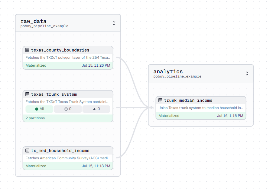
Here we can see our DAG aka our Directed Acyclic Graph representing the network of our software defined assets.

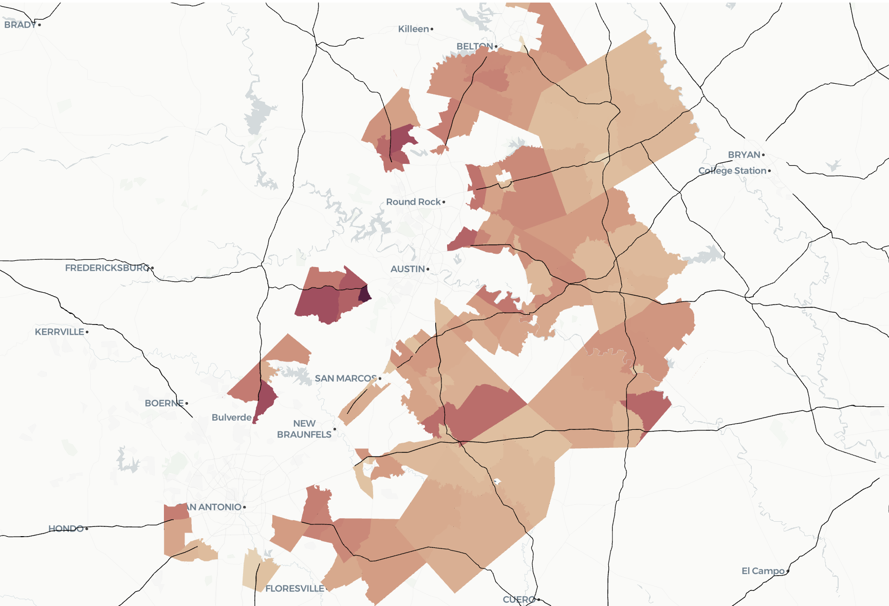
And alas, here's what we've produced (median household incomes rise from light to dark).

Try it out

All this code can be found on GitHub. Feel free to clone the repo and try it out for yourself.

GitHub - alexlowellmartin/poboy-pipeline-example: Building a po’ boy’s spatial data pipeline from scratch with Dagster, geoparquet, & R2. (This is an example)

Building a po’ boy’s spatial data pipeline from scratch with Dagster, geoparquet, & R2. (This is an example) - alexlowellmartin/poboy-pipeline-example

GitHubalexlowellmartin

Up next

This is just the very just the start of this pipeline build. We addressed only one of a handful of common source systems. We mostly only went one layer deep (getting data in the door to our landed layer). And we only addressed spatial data forked into R2 as GeoParquet.

Here's what I'd like to tackle next, in a somewhat particular order:

• Add unit testing
• Build a NAS resource
• Incorporate existing DuckDB / MotherDuck I/O managers
• Build out resources for MapServers, WFS, WMS, Shapefile, KMZ, KML, and GeoJSON downloads.
• Extend our R2 resource to handle other spatial and tabular use cases
• Implement dbt to handle transformations
• Fetch a bunch of the most relevant datasets and, from those, start building enriched datasets

Adios.